Propeller Application
Erik Skarman
Firstly
This is a new version of this page. Many things are updated
here. Most of all, I am using a new language, called
MPS. Many of the applications are new or updated too.
Many of the files can be downloaded from the
chapter MPS objects
The old version is available
here
The Propeller microprocessor
The Propeller microprocessor is a computer developed
and produced by Parallax Inc. It is a 32 bit computer
running at 80 MHz. Its most important feature is that
it has eight individual processors, called cogs,
which operate in parallell. When all these processors
are working, the total capacity of the machine is thus
640 MHz.
More importantly, however, the eight parallell processors
allow you to work easily and nicely with real time
systems, controlling and interacting with "real things".
You can avoid the interrupt concept, with all its
pedagogical difficulties and pitfalls. Instead,
you assign a dedicated processor to monitor events from,
say, a sensor. When it detects the event it can grab
some external signals and then invoke computations in the
other processors in a very versatile and transparent
way. For the monitoring there are instructions that
monitor an event in a single instruction, so that the
computer stays within the instruction until the event
happens.
The processors communicate with each other over a global
memory. This memory is connected to the processors in a
round robin fashion, thus avoiding the risk that two
processors try to access the memory simultaneously.
To allow constistent transfers of data chunks with more
than one word, there is a semaphore concept.
The processors communicate with the external world over
32 I/O pins which are programmable to be either input or
output pins. There is a simple scheme for resolving
conflicts between several processors accessing the same
output pins. All input pins are simultaneousy available
to all processors.
The processor also has a real time counter, running through
all the values of a 32 bit word in a few minutes (after which
it overflows and restarts), and
wait instructions that halt the processor (cog) until
the time counter has reached a specified value. In this
way it is possible to contruct very accurate real time
functions.
Content
Programming languages
Propeller Assembler
The Assembler language of the processer is
available to the user through the Propeller Programming
Environment (even though in some sense it has to be
encapsulated in a Spin program). Here is a sequence of
four instructions which can illuminate some special features
of this assembler language:
sub x,y nr,wz
if_eq mov x,y
if_eq jmp #zero
if_neq jmp #nonzero
Here we subtract the variable y from the variable x,
The result would be stored back in x, but not in
this case, due to the nr flag (no result). Instead
the wz flag commands an update to a z-register. This
z register becomes true if the result was exactly
0 and false otherwise.
The next two instructions are gated with this. They are executed
only if the z-register is true. First we move the value
of y to x (which is kind of meaningless, because in this
situation, x and y are already equal). Then we jump
to an instruction labeled with "zero".
If the z-register were false, the two first instructions would
be executed as no-operation-instructions (nops), and then
the program would execute a jump to the instruction labeled
with "nonzero".
The z-register has a sister, the c-register, which indicates
whether the MSB of the result is 1, but it can also
detect overflow.
This gating of instructions with conditions allows
the building of "if-then-else" constructs without
using jumps.
Spin
The Propeller computer is supplied with another
language at a higher level, the Spin language.
It is an interpretive language. This means that the
programmer is not running his own code. He runs an
interpreter, resident in the propeller, which interprets
the Spin code (somehow encoded into 1:s and 0:s).
This interpretive principle facilitates the design of
a nice high level language. But the whole method is slow.
Given a high level Spin language and a fast Assembler language,
the natural approach would be to write time critical
functions in assembler, and connect them through a Spin
program. To my understanding, this is not the way Spin
and assembler code work together. The Spin "call" to
Assembler code amounts to that a cog is started to run
from the machine adress of the indicated assembler code.
But there is no return instruction to return to the Spin
code.
MPS
After some time with the Myra language, that you will find
here, I decided to go back to an older
language idea. The purpose was to get smaller and faster
programs, by working against a computer model that was
closer to the real architecture of the Propeller. Speed
may be important, but program size is even more important in
Propeller applications, because of the relatively small
memories in the Propeller cogs. In fact, the size is only
496 longwords. It may seem pretty hopeless to solve any
task with such a small program size. But, after all, you have
8 cogs of this size, and in these types of computers you can
do a lot with small programs.
You find a more or less complete
documentation of the MPS language, and also the standard
object file std.mpo
here
For Myra, I decided to make an interpretative version, to
overcome the progam size limitation. For MPS I haven't done
that. It seems that I can solve my problems with the standard
language. Myra also made use of an assembler resource file
written in assembler, but for MPS I don't need that.
I can write everything I want in MPS, except for a few
lines with so called in line assembler code.
The MPS system
Here is the software you have to download in order to
use the MPS language:
- MPS.java.
This is the
compiler for MPS. Download this and the other
java files, and then compile using the javac Java
compiler. Run as
java MPS mpsprogram
where the filename extention '.mps' is left out.
The compiler will produce a number of spin code
files. The first of them will be called mpsprogram0.spin,
and it contains the program for cog 0, which will then
load the other cogs. Normally the other files are
called mpsprogramM0.spin, where M is the number of
the cog. If several programs will be run in one
cog in series, there will be names like mpsprogramM1,
mpsprogramM2 etc.
Open the Propeller environment or the
Propellent environment with the file mpsprogram0.spin.
From there, the code can be loaded into the Propeller.
-
Propasm.java. This is an
assembler, which creates machine code from
assembler code. The machine code is not currently
used, but the file Propasm.java has to be available
anyhow.
- codes.txt
contains binary instruction
codes for the assembler instructions. You can augment it
with missing instructions, to help Propasm handle
more programs, but note that some instructions
are distinguished by bits outside the instruction
code proper. This file is used by Propasm.java, so
it needs to be in place.
- conds.txt
contains binary
codes for the different conditions if_a, if_nz etc.
- InFile.java
encapsulates
java's file concept to create an input file.
- OutFile.java
creates a java output file.
- Text.java
contains
stringoperations acting on an object Text which
encapsulates java's String concept.
-
StringOp.java. This
is an older system for string operations, that is
used in the older programs InFile and Outfile.
(Sorry for that some of java files are commented in
Swedish. I don't think yo need the comments, but if you know
Swedish, they may be of some help.)
MPS.java starts with
a comment block, which describes the hierarchy of methods.
In the right collum, there are designators for the methods,
and these will reappear at each method, so you can find
the methods by searching for these designators.
MYRA
An interest I had in stack programming several years ago,
led me to try to design a stack based higher level
language, that could be compiled into assembler. I was
also inspired to this by someone, who had made a FORTH
programming language system for the Propeller. FORTH
is a stack based programming language, and so is my
language, called MYRA. A documentation of this
language is found here.
I had some introductory comments on Myra here, but I have
now removed them.
The Myra System
Here is the software you have to download in order to
use the Myra language:
- Myra.java.
This is the
compiler for Myra. Download this and the other
java files, and then compile using the javac Java
compiler. Run as
java Myra myraprogram
where the filename extention '.myr' is left out.
The compiler will produce a number of spin code
files. The first of them will be called myraprogram0.spin,
and it contains the program for cog 0, which will then
load the other cogs. Normally the other files are
called myraprogramM0.spin, where M is the number of
the cog. If several programs will be run in one
cog in series, there will be names like myraprogramM1,
myraprogramM2 etc. The compiler has a boolean called
machineCode. If this is set to true, Myra will
generate machine code, for the cogs from 1 and up,
though this machine code will be disguised as
assembler code in the form of variable declarations.
In this case, the Myra compiler will print the
number of memory cells used in each cog. If any of
these numbers exceeds 496, the loading of the program
will fail. Open the Propeller environment or the
Propellent environment with the file myraprogram0.spin.
From there, the code can be loaded into the Propeller.
-
Propasm.java. This is an
assembler, which creates machine code from
assembler code. It is only used when Myra.java
has its machineCode boolean set to true,
but it is needed to make Myra.java compilable in any
case. It assembles code from the file Program.asm
to the file Program.bin. It is not a complete assembler.
It only handles the assembler operations that the
Myra system generates.
- Disasm.java.
This is a
disassembler from machine code to assembler code.
It is not a part of the system, but I made it to
help debug Propasm.java.
- codes.txt
contains binary instruction
codes for the assembler instructions. You can augment it
with missing instructions, to help Propasm handle
more programs, but note that some instructions
are distinguished by bits outside the instruction
code proper.
- conds.txt
contains binary
codes for the different conditions if_a, if_nz etc.
- InFile.java
encapsulates
java's file concept to create an input file.
- OutFile.java
creates a java output file.
- Text.java
contains
stringoperations acting on an object Text which
encapsulates java's String concept.
-
StringOp.java. This
is an older system for string operations, that is
used in the older programs InFile and Outfile.
- Assembler.spin.
This is the assembler resource file, which contains
a diversity of usefull (and in some cases indispensible)
assembler routines. Your are welcome to add new
assembler routines to this file, once you have learnt
how to do it.
- Macros.myo.
This is a small file that contains some macros, that can
be substituted into the Myra code.
- Patterns.myo.
This is as yet an insignificant little file, that
contains (so far) one software pattern; a
system for iterating through the elements of
an array. It is used by the file display.myo.
(Sorry for that some of java files are commented in
Swedish. I don't think yo need the comments, but if you know
Swedish, they may be of some help.)
Myra.java starts with
a comment block, which describes the hierarchy of methods.
In the right collum, there are designators for the methods,
and these will reappear at each method, so you can find
the methods by searching for these designators.
"A Propeller ecology"
As a little apetizer for the rest, I will present the
following figure, which displays a Propeller surrounded
by devices, from which it can get sensory data and operator
commands, and on which it can act. In short - an ecology
around the propeller:
Let's start in the upper left corner, and go around in
counterclockwise direction.
In the upper left there is an analog to digital converter.
To it, we can connect potentiometers, and thus control the
program with one or more knobs. There is also a great
selection of sensors, that give analog outputs. In the
figure we have shown gyros, which measure rotation, and
accelerometers which measure acceleration and tilt (due to
gravity). Under the A/D converter, there is an RGB LED on
which we can create colors. Its main use is perhaps for
debugging. You can display a certain color, when you come
to a certain point in the program.
The next item is a keyboard, which can be used to control
a program. Here I show a numeric keyboard, which is smaller
and handier than a full alphanumeric keyboard. Touch controls,
which play such an important role in smartphones, are
available to amateurs today, but perhaps only in the older
form of resistive touchscreens, which require using
a stylus. With a touchscreen, you can make a universal
mode selector, by drawing "buttons" behind the screen, or
you can input analog data. You can relatively easily make
a program to input simple sketches to your computer.
RFID is a way to recognize simple and cheap "tags", when
they come into the vicinity of the RFID device. Each tag has
a unique serial number, and you get that, when the tag is
detected. One, maybe bad, idea I had about this, was to use
RFID for robot navigation. You placed out tags, and when the
robot encountered a tag, it would know where it was.
"TCP/IP" represents a little device called WiFly, which
lets you connect your Propeller to you WLAN at home. From
there you can go with your Propeller data out on the world
of internet. ZIGBEE represents a wireless device, so that
you can send data (and commands) between your Propellers
wirelessly.
The EEPROM is an integrated part of the Propeller system.
That's where you store your program, if you want it to
be started after power down/power up. All that is programmed
into the Propeller. But you can write you own code, to talk
to the EEPROM, for your own purposes, and you can stack more
EEPROM chips to the same wires, to get more space for data.
I have also tried some other components with the same
functionality, but with more capacity. They are usually
called flash memories, but they are functionally EEPROMS
(Electrically Erasable Programmable Memories).
RAM is a Random Access Memory, i.e. a standard memory, where
you can store data at high speed. But you loose the data
at power down. A RAM has many pins, so I have chosen to
connect the RAM via an interface Propeller.
SD is an SD-card (Secure Digital). Technically it is a
flash memory and a small interface computer, built into
a "card" that you can plug into a slot. They have a huge
capacity, and it is practical that you can plug them
in and out.
ESC is an Electrical Speed Control, which belongs to the
world of Radio Control Aircraft. You connect a powerfull
battery to the left, and a brushless motor to the right,
and then you can control great mechanical power with pulses
from the Propeller.
Over that, there is a more conventional way to control
standard DC motors with a so called H-bridge.
The diodes further up
belong, together with the striped strip, to an
odometry system. With that you can measure displacement along
the strip.
The, maybe, camera like object at the right top, is
- a camera. It is a camera with a serial interface, so that
you can get the pixels of the picture into the computer.
The rectangle with the sailboat is a graphical display, with
color depth good enough to display photographs.
But, with some programming, you can also display
alphanumerical data on it.
Finally, the USB box, is the standard umbillical through
which the Propeller is loaded with programs from a PC.
But you can also use it to up/download data from/to the
PC. You need some software at the PC-side to take care
of the data. Such a program will be presented
here. Concretely the USB box
contains a little device called a Propstick.
With that and the Propeller development environmens,
you can load programs into the Propeller.
Given all this, you can build different combinations. For
example, if you take a picture with the camera, you would
like to store it on the SD-card. But for most cameras,
the camera produces more data than you can handle in time
with the SD-card. So you may need to store the picture
in the RAM. After you have transferred the picture to the
SD-card, you can display it on the display at any time.
Hardware considerations
Analog input
The propeller computer doesn't have any analog inputs.
Its cousin, the Basic Stamp, handles analog inputs by
means of RC circuits, which convert analog voltages to
times. Times can be measured accurately with both
Basic Stamps an Propellers. So I guess, one can use
a similar design for the Propeller. However, one needs
one pin for each analog input, and probably one more
input to discharge, or precharge the RC-circuits.
So my alternative has been to use separate A/D converters.
My favorite is Microchip's MC3208. It converts 8 channels
to 12 bit digital data. It has a serial interface. You
need to handle a chip select pin, a clock pin, one data-in-pin
and one data-out-pin. So for 8 analog channels, you need
4 pins. If 8 channels aren't enough, you can get 16
channels for 5 pins etc..
You send a conversion order to the converter's data-in-pin.
This order announces which channel should be converted. Then
you can clock your digital result from the converter's
data-out-pin. All this is done in a function adc.get
in the file adc.mpo. The call is like this:
( channel )adc.get ->x
The result appears in the 12 least significant bits in x.
"channel" of course is the number of the desired analog
channel to the MC3208.
The system needs to be initialized with
)adc.init
That function is also in adc.mpo. This function assumes
that the converter is connected to the first four pins
of the Propeller in the order they appear on the chip.
Unlike what I have said before, MC3208 doesn't need
5 volts. It can run on 3.3 volts. In case you connect it
to 5 volts (which gives you a slighly lower noise level)
you need a resistor of some kohms between the converter
output and the Propeller. Otherwise you will destroy that
pin on the Propeller.
Analog output
A parallell input Digital to Analog Converter (DAC)
would require many Propeller pins, but I have a
serial interface DAC called MCP4822, and I have made
an mpo-file for it:DAC.mpo. It is a small power
device, so you may need to add some power amplifier to
it.
But another popular way to make analog outputs is with
PWM, pulse width modulation.
There is a pulse repetition
frequency (prf) for the pulses. Then the pulse is on
for some percentage of the total period, and off for the
the rest. Afterwards, you can remove the pulses with
a RC-circuit, and just keep the average, which will
be an analog signal. But if the output goes to, for instance,
a motor, the motor can filter out the pulses with its
mechanical inertia. In that case, you may need to
raise the prf to well over 10 kHz. Otherwise you will
hear the prf from the motor. The time constant of the
RC circuit or the motor will limit the bandwidth of
the output. You need a margin between the desired bandwidth
and the prf, but for mechanical systems, this is usually
not a problem.
Here's an example. We want to control two
motors, and we want to drive them in both directions.
Assume that we connect motor 1 between pins 0 and 1,
and motor 2 between pins 2 and 3. We can drive the motors
with codes like this:
- 0001: Motor 1 forward
- 0010: Motor 1 backward
- 0100: Motor 2 forward
- 1000: Motor 2 backward
- 0101: Both motors forward
- 0000: Both motors halted
- etc.
In order to control two motors simultaneously, we can
use two processes, which is simple. But if we need to
save processes, we can control the two motors with a
single process. Here comes some MPS code for this.
We have two velocities v1 and v2 for the two motors. They
are scaled so that 255 means (almost) full speed, and
0 means no speed. In some cases we have to avoid full
speed for hardware reasons (more about that later). Now
let ttot be the time of the full period. Then we can
compute an on time like this:
ttot *v >>8 ->ton
The shift by 8 is a division by 256, to remove the scaling
of the v variable. Multiplication and shifting must be done
in this order. Now, we can save computation time here, by
letting ttot be an integer power of 2. We can choose ttot
as 4096, which is the 12th power of 2. So, now the multiplication
can be replaced with a leftshift with 12. Then the whole
first equation can be replaced with:
v <<4 ->ton
This is good, for it reduces the time, we have to keep the
motors idle. The value 4096 gives a frequency of 20 kHz which
is not hearable for (most) humans. The direction of motion
is given as two masks m1 and m2. We need a program that
turns the motors off at the right time. Now as we control two
motors
at the same time, we can't use the wait instructions,
so we have to check the computers real time clock cnt
and use if-statements instead. Here's the code
process pwm
ttot = 4096
begin
( $F )setdir
:loop
v1 <<4 ->ton1
v2 <<4 ->ton2
( m2 <<2 |m1 , $F , )outpins
now ->t0
:tloop
if(now -t0 >ton1){ ( 0 , $3 , )outpins now +ttot ->ton1 }
if(now -t0 >ton2){ ( 0 , $C , )outpins now +ttot ->ton2 }
if(now -t0 >ttot):loop
A:tloop
The mask $3 directs the outputs to pin 0 and 1 where
motor 1 sits, so we can turn motor 1 off with that. The
mask $C does the same for motor 2. And the mask $F
is used to turn both motors on. Note that the instruction
now loads the real time counter cnt. v1 and v2 and
m1 and m2 are global variables computed elsewhere. m1 = 1
means that motor 1 is driven forward. m1 = 2 drives the
motor backwards. We could also use m1 = 0 if we want to
hold the motor entirely. Note that the motors are held
while we compute ton1 and ton2.
Power drivers
We now want to connect power drivers to the Propeller
output pins, and connect the motors between the outputs
of the power drivers. This structure is sometimes called
an H-bridge.
TDA2050
Here's a solution based on an integrated circuit
called TDA2050:
TDA2050 is marketed as an audio amplifier, but it
is actually a universal operational amplifier, with
capability to deliver high power. It amplifies the
difference between the + and --inputs with a gain
of one million or so. Then we can reduce the gain
with a feedback through the resistors R2
and R1. We would like to create a gain
of about four, to increase the 3.3v span of the Propeller
to an output span of 12v. But with the TDA2050 you can't
reduce the gain that much without getting oscillations.
A gain of about 40 is minimum. So we live with that, and
reduce the input signal first with RI and
RT.
RC and CC make up
a capacitive load, also to enhance stability. The
capacitor CV shall eliminate spurious feedback
between the different steps of the amplifier over the
12v supply rail. It should be placed physically close to
the circuit.
The capacitor CT together with (essentially)
RT helps remove the pulses from the PWM-system,
and just keep an average.
We have time constant of appoximately 500μs, which should
filter out the pulses with a period of 100μs pretty well.
At the same time, such a time constant shouldn't cause
any stability problems for the mechanical system.
The question is still, if the capacitor CT should
be there. With the
capacitor in place we avoid hearing a tone from the motor.
At least cats may appreciate that. Perhaps we save the
motor from some wear. And we avoid disturbing the electrical
environment around our device. The penalty for all this
is heat dissipation.
Without the capacitor, we drive the TDA2050 in full
saturation all the time. The output transistors are either
fully on or fully off, and hence consume no power.
However, such operational amplifiers are not so fast,
so they spend some time in the transition phase, so
some power is still dissipated.
With reasonably small motors, both solutions should work,
but you need a heatsink for your amplifier, and free
air flow round the heatsink. TDA2050 and many other
modern circuits have the advantage that the cooling
tab is connected to ground, so you can without risk
screw all the circuits firmly to the same heatsink.
IR2103
An alternative for even higher power is to use
a IR2103 circuit, which is a FET-transistor driver from
International Rectifier. Here's a quick sketch of how
it is connected.
To drive the upper FET to open, you need a gate voltage
a few volts over the drain. So to bring the output all
the way up to the E volt rail, you need more voltage than
E somewhere. In fact, the upper FET is
driven by a little circuit, that sits between the
terminals O and X. X should be 12 volts higher than O.
The question is, how we get that voltage there.
A hint is to think about a so called charge pump, as
in this figure:
C1 and D1 will clamp the voltage
at P never to be under the rail voltage. (12 volts).
Consequently
the voltage at P will vary between 12 volts and 17 volts
(as 5 volts is the amplitude of the oscillator).
D2 and and C2 will rectify and smoothen this
signal to give a voltage 5 volts over the 12 volt rail.
This works fine, but it probably doesn't work
unmodified, if we are going to pump a voltage over
a rail, that moves all the time. That is the situation
we have with our IR2103 circuit.
The conventional way to provide the X voltage
is to use the systems output signal as charge pump
oscillator. Here's the way it is done.
When the output O is all the way down to zero, the
capacitor C will be charged through the diode D.
Then, when O flies up, C will fly up with it. It
will gradually discharge, though, so O will have to
go down to zero every now and then. This is a constraint
for the programming of the device. With the PWM, the
pulse width must never be 100% of the full period.
This is OK, but it may be easy to forget, when you
make your programs.
Hence it would be nice if we could design a system
with an independent oscillator for the charge pumping.
It's open for invention. With a little luck, we could
maybe use one oscillator for all IR2103-circuits around.
IR2103 is a purely digital system. The input is truly
digital, so there is no way, that you could smooth
away the pulses with capacitors. The circuit is fast,
so the time in transition between the two saturated
states is short, and the switching is also synchronized,
so that both FET:s are on simultaneously only for very
short periods.
The most dramatic property of this circuit is, however,
the bound on the voltage E. E can be as high as 600 volts!
With 600 volts supply, these 600 volts penetrate right into
the IR2103. It's a tiny 8 pin dip-circuit, or an even
smaller surface-mount version, but it is said, it can
take it. Beware however! Your circuit board design might
not tolerate 600 volts. Maybe you dare to work with
200 volts. You easily find FETs that can handle 7 A (with
some cooling). Then you can control 1.4 kW power from
a 3.3v output from a Propeller pin. That's pretty awesome.
Integrated power drivers
Lately I have had some problems with the IR2103 driver,
in that some of the FET:s have been destroyed. I don't know
why, but it always hard to remove and replace components.
Because of this, I have tried another alternative. It is
an integrated driver called L298. It contains two full
bridges (4 half bridges), so you can drive 2 DC motors
(or 1 stepper motor) with it. It comes as a so called
Multiwatt package with 15 pins. The circuit works fine,
and I have been surprised that the component stays so
cool. You can mount it on a bit of aluminum profile, if
you just drive moderately sized motors. The circuit can
drive up to 48 volts and a few Amperes.
Another circuit is called L293. It is an ordinary
DIL20 capsule, which is a little more difficult to cool.
It has four ground pins, and you can make a larger suface
on the circuit board connected to the ground pins for
cooling. I haven't tried these circuits yet, but they are
part of an Arduino motor shield, and also of a Raspberry
PI motor interface.
Protection diodes
Electrical motors have an inductance. Then, when you
stop the current through the motor, the inductance will
respond with a very high voltage. This could destroy your
electronics, so you need to have protection diodes to absorb
the voltage peaks. The choice of these diodes is a little
mysterious. International Rectifiers driver FET:s
(called among others IRF510) contain protection diodes,
so the problem is solved there. For L298 you have to add
diodes yourself. I have the impression that they are built
in into L293, but I am not sure. An important factor is
that they are fast. When you reverse the voltage over a
diode, you expect that it would stop conducting. But before
that, the charge carriers have to leave the diode. In a
standard diode, there is no electric field at this occasion,
so the charge carrier leave by diffusion only, and this
takes a loooong time (a few microseconds). (There is the
same mechanism in bipolar transistors). Shottky diodes have
another desigh that overcomes this. The measure of this
is called trr (reverse recovey time). You rarely find this
information for slow diodes, so look out when this is not
mentioned. As there weren't many enough fast diodes in
stock with my supplier, I tried a fast but small diode
called 1N4148 (a classical diode). I put two in parallell, and
it seems to work fine. My recomendation is still to look
for somewhat bigger Shottky diodes. Here's a circuit diagram
for how to connect them:
Here's a picture of a motor driver circuit based on
integrated power drivers:
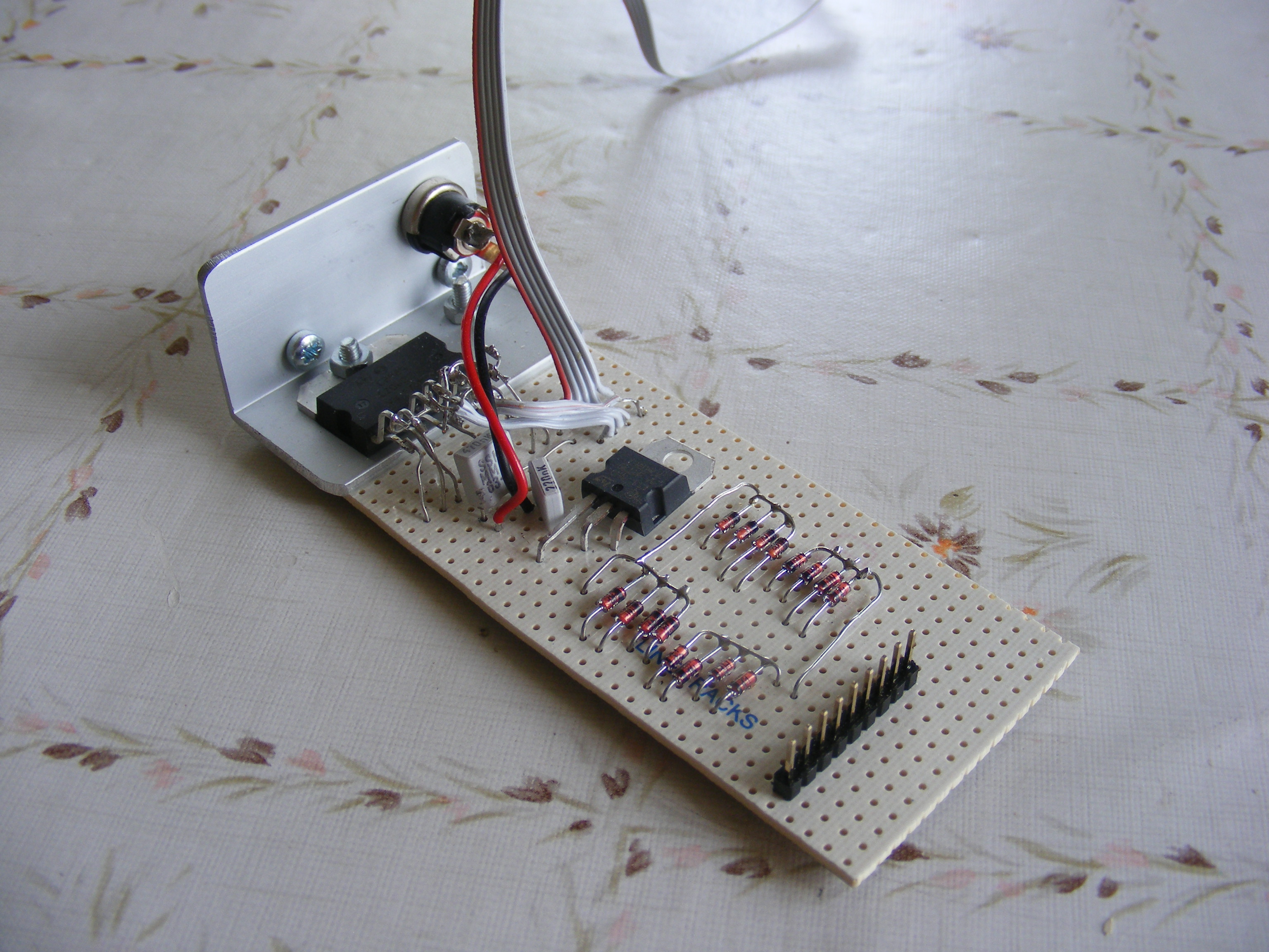
The integrated circuit is to the left. I have chosen to
connect it in a pretty primitive way with wire to make it
easier to replace when necessary. Then you see a 5v stabilizer
for the logic level of the circuit, and then the protection
diodes.
Motors
DC-motors
(Most of this applies to AC-motors as well, but DC-motors
are more popular in control applications.) As just mentioned,
a motor has an inductance (it has a coil in it), and this
means that the motor produces high voltages if you try to
stop the current through it quickly. So use diodes as
presented previously.
Secondly, a motor is also a generator. So it produces a
voltage proportional to its rotation speed: ug
=a·ω.
It is the difference between the applied voltage, and this
generated voltage, that drives the current through the
motor winding. So the current i = (u-ug)/R,
where R is the resistance of the motor winding (usually
a small value).
Then that current determines the torque M of motor:
M = b·i. This torque is then reduced by external torques
Mext,
like friction. This gives an acceleration of the motor
as dω/dt = 1/I·(M-Mext), where I is the so
called moment of inertia of the motor + what is connected
to it (this becomes a bit complicated, if there is a gearbox).
Now, let us think that Mext is small, so that
motor is almost free wheeling. Then the motor will keep
accelerating, and ω will grow, and so will ug.
Finally, the current will be very small, but the torque
M will manage to balance, the small Mext. So
we have the equation u-ug ≃ 0, or u - a·ω ≃ 0, or
ω ≃ u/a. So, the voltage over the motor controls the
motor's speed.
Now, let's grab the motor axis and hold it firmly, so that
the motor stalls. Then ω = 0 and ug = 0. So
the current is u/R, which is a high current. This current
controls the torque of the motor. This is the torque, that
we feel in our hands, when we try to stall the motor.
So now the voltage of the motor, or the current through
the motor controls the torque.
Hence the motor acts somewhere between two extreme modes,
one where voltage controls speed, and another where voltage
controls torque. We can also see that the motor is not
a passive receiver of electric signals. It responds by
requiring high currents if it experiences mechanical
resistance. Finally, if you make some kind of
feedback to your motor, from, say, the position of the
motor, the generator effect in the motor will contribute
with some damping, which you probably very well need.
Brushless motors
Brushes in a motor serve two purposes. They bring
the electric current over to moving coils in the motor.
And they serve as so called commutators, which reverse
the current, when the motor has gone a half turn. To
get brushless motors, you have to do two things. First,
you build a motor with stationary coils, and a rotating
permanent magnet. Then you have to solve the commutation
problems.
You can simply drive the motor with alternating
current. With some luck, you can have the motor rotate
in sync with that alternating current. In order to drive
the motor in one, and only one, direction, you should have
a three phase system, but you can create a false third
phase with a capacitor.
Another idea is to measure the
position of the motor with a sensor, and then
reverse the voltage with electronics at the right moment.
This is a kind of "software commutator". But then you can
maybe avoid the separate sensor, by registering the
motor voltage. There will be a small pulse induced, when
the moving magnet passes one of the electromagnetic poles,
This is not quite easy, because you are trying to measure
some small induced voltages, while you are, yourself, imposing
much higher voltages. But it can, obviusly, be done.
After all this, the motor is simply a three phase motor.
And the electronics is a machine for creating three phase
alternating voltage based on
- How the motor responds to the signal.
- What the operator wants from the motor.
This is an ESC, an Electronic Speed Controller. It's
admirable stuff! You can get high speed and hight torque
out of such a motor, and it is easy to control. You tell
it what you want in terms of a regular pulse train, where
the pulse length declares what you want.
The question is: What is it that you want? The specifications
for these devices are not very clear on this. That pulse
width doesn't determine the speed only. At high mechanical
resistance, the motor goes slower. Another thing that you
would like to see specified, is the dynamics. How fast does
the motor go up to the final speed? There is also some
logics, that may make the motor wait a little while before
starting. All this was crucial in my application: A helicopter
with four rotors. I failed with this project. Since then
I have tried to measure the dynamics of these devices, and
maybe I will return to the project after having analysed
this.
But if you have less dynamically critical applications,
brushless motors together with ESC:s can be a good
alternative.
Stepper motors
A stepper motor moves in steps. These steps are steps
in position, so they are in themselves position controlled
devices. You can control their speed, but hardly torque.
The idea is that you can send a sequence of positive
and negative voltages to (usually) two windings. Such
a sequence will take the motor 4 steps, but you can stop
anywhere in the sequence. Then the motor will stop where
it is. You basically have full control of the motor.
By running through the sequence at a defined pace, you
can get a specified velocity.
A stepper motor has a hold torque. If external forces exceed
that torque, the motor will slide away. If you thought that
you would have full software control of where the motor
is, this is a disaster. The holding torque is a function
of the current you send into the motor. Higher current
means higher holding torque, but at some current, the motor
will overheat. Now, here's a disadvantage of the motor.
If we want a reasonable holding torque, we have to send
a hight current into the motor all the time.
For some applications, where the motor is connected to a
big inertia, stability may be an issue. The motor might
slip over a lock position and go to the next.
A stepper motor normally has two coils and a rotating
permanent magnet with many poles. First one coil attracts
a north pole, while the other is passive. Then you can
remove current from the coil, and apply current to the
other. Then it will attract the north pole. In the next step
you reverse currents to attract the south poles instead.
After 4 steps you can repeat the pattern, to attract the
next north pole.
Obviously you need 4 power amplifiers here, to drive
a stepper motor. With these amplifiers you could otherwise
run 2 DC motors in both directions.
So the issues with stepper motors are:
- Is the hold torque (based on the maximum
tolerable current for the motor) enough for
the mechanics of my application?
- Can I deliver the required current to the
motor continously?
The object file Stepper.mpo contains functions to
be called in the following way:
( motorpin1 , motorpin2 , )step.init
)step.drive
)step.drive2
motorpin1 is the lowest pin number for motor1,
and motorpin2 is the lowes pin number for motor2.
The rest of the 4 wires from each motor should be connected
to the pins next to the lowest pin. The two wires belonging
to one and the same winding, should be connected to
consecutive pins. If you are unlucky, the motors might go
in the wrong direction, and in that case you might have
to change the wiring. The function step.drive2 is made for
driving two motors. If you only use step.drive, it is
unimportant which value you assign to motorpin2.
The motors are controlled by one or two global variables
xc or xc and yc. The motors move to the
rotational positions xc and yc. The
functions step.drive and step.drive2 are infinite
loops, so the process can just call them, and then it
won't be returned to. So here's what a process might look
like:
process drive
begin
( xx , yy , )step.init
)step.drive2
load from (stepper.mpo)
*step.init
*step.drive2
\
Communication
RS232
RS232 is a very old protocol for communication. It has
changed name now to EIA232, but very few people seem to
have noticed that. It is a standard for serial communication
over only one line (per direction), where the bits
are sent after one another in time. It was fairly specific
about voltage levels, and it had several options for flow
control, so that a receiver could inhibit data sending,
when it was too busy. Surprisingly for a one line concept,
the protocol was standardized for a 25 pin D-sub connector.
The standard was also pretty open, when it came to
different parameters like number of bits sent, parity,
sign on start bit, communications speed etc..
Luckily a certain set of parameter values have become
de facto standard, so now we communicate with
a large number of devices and modules, with almost the
same communication parameters. At the same time, the
voltage level issue has become less important. Most
devices use 0 volts as 0, and 5 or 3.3 volts as 1. But
if you buy a true standard RS232 device, and connect it
to a Propeller computer, the Propeller will be destroyed,
as the voltages are too high.
If I can, I always avoid flow control, as it complicates
things (more wires, more Propeller pins used etc.) Most
devices can be configured so that flow control is not used.
The standard allows parity control, but the most common
choice is "no parity", which simplifies your software.
You don't need to set parity bits, and you don't have
to check them (you never have to check them, even if
they are there).
The most common communications speed nowadays is perhaps
115200 bits per second, which is about what today's processors
can manage. But the default setting is often 9600.
Conventionally these bit rates are called baud rate,
and the unit is baud, and not bits per second. So we
have 115200 baud etc. (The reason for this is that the
term bits/second is reserved for the effective speed
of a line with disturbances. If there are disturbances,
you have to check and resend, and you loose speed on
that.)
Some devices can tell you which baud rate they are set to,
but if you don't know the baud rate, you can neither put the
question, nor interpret the answer. Most devices have
some sort of reset button, which restore default parameters,
like 9600 baud. For the eventuality that you
have abandoned the default parameters, and happen to
press that button, you have to have a little reconfiguration
program up your sleeve. This is a maintenance problem
for your system.
Then, the normal standard is that the line is 1 when it
is idle. A new transmission is announced by the line
falling to 0. This is the start pulse. Then you wait
one and a half of TS, where TS is
1/(baud rate).
Then you can clock in yor data every TS, least
significant bit first. The standard is that one such package
of bits is 8 bits long. Then follows an optional parity bit
and one or more stop bits. When it's all over the line
goes up to 1 again. It is not terribly complicated to
build and read such a pulse train, if you have computer.
To do it with conventional hardware was probably quite
complicated.
As RS232 is such a common protocol, I've put the code for
it in the standard object file std.mpo.
The standard routines are called as:
( data , pin , pulse , )send
( pin , pulse , )receive ->data
pin is the pin to which you have connected the wire
to the other device. pulse is 1/baudrate, but
expressed in Propeller tics. So with the standard setup
for the Propeller with a 5 MHz chrystal and a PLL of 16,
for a baud rate of 115200 you should set
pulse = 80000000/115200
The receive program is blocking, i.e. you get stuck in there
until some data comes. You also have to be in that program
almost all the time, to be alert, when data arrives. This
means that that function needs its own process.
There are versions for 9 bits called send9 and receive9, which
are called the same way. And there are versions for 32
bits word length, but they are called without the variable
pulse, as they assume a default baud rate of 500000.
I2C
I2C is a bus standard invented by Philips. I2C means
Inter Integrated Circuits, and is thus a bus for communication
between individual circuits in an electronic system. It is
a master/slave concept, where a master controls the
trafic on the bus. In the general case, there can be more
than one master on the bus, which calls for an arbitration
policy to divide the bus between the masters. However, in
most cases, there is only one master.
The bus has two wires, one data line and one clock line.
The slaves and the masters are connected with open collectors.
Consequently, when a device tries to send a '1', the collector
is open, and thus, the impedance is infinite. The voltages
are pulled up with a set of pull up resistors, which belong
to the bus.
The role of master in our application, will most likely be
played by a Propeller computer. The Propeller doesn't have open
collector outputs, but we can mimic this by using the
direction register. We permanently set the output to the
pin to zero. When we direct the pin to be an output pin,
zero with low impedance will be visible on the pin. When
we direct the pin to be an input pin, a high impedance is
visible, and the pull up resistor of the bus will pull
the line high. When we expect inputs from the line, we
should set the pin to 1, i.e. high impedance. When we send
data to the device, we should expect an acknowledge signal from
the receiver. At that moment the master should have high
impedance, but there is no harm if we forget that (except
that we mislead ourselves to beleive that the acknowledge
signal has come).
Data are clocked by the clock wire in the sense that the
slave can trust the data, when the clockline is high. Hence,
the data line should not change, when the clock line is
high. If it does, this is taken to be a start pattern or
a stop pattern. When the start pattern appears, the
slaves should expect data on the bus. The first data
after the start pattern is a device adress (plus a read/write
bit). Those slaves which do not recognize the adress as
their own, can now go to sleep, and they don't need to wake
up again, until a stop pattern appears. Communication is
now open between the master and a single slave, and the
way the communication proceeds is pretty much an agreement
between the two. What normally happens, is that the master
sends data to the slave. If it wants to receive data from
the slave, it normally sends a new start pattern and
the adress, but now with a read bit. When one of the sides
receives a piece of data, it acknowledges this with a single
zero on the data bus.
The I2C protocol has an object file called iic.mpo.
Its functions are called in the following way
( clockpin , datapin , )iic.init
)iic.start
)iic.stop
)iic.ack
)iic.wack
( data )iic.send
)iic.rec ->data
iic.ack will clock out an acknowledgement signal
(=0) as a master is expected to do it. iic.wack
will clock in the acknowledgement from the slave. The
result will be returned. It should be zero, but you may
skip checking that. But you do have to run iic.wack after
you have sent data, because the slave needs the clocking
to go on.
This is the basic protocol. You use iic.send also
to send the slave adresses. But you have to consult the
specification of your device, to find out which adresses
and data you should send.
The iic-object is intended for making master software.
To be a slave is actually more difficult. because you
have to recognize start and stop patterns, and this is
not supported by this object.
We will come to an application of the I2C bus in
the radio application.
Also, the Propeller standard EEPROMs use the I2C bus,
and there are many sensors that use it too.
Formally, when you use
the I2C bus for comercial use, you should pay
a license fee to Philips.
SPI
SPI means Serial Peripheral Interface. Unlike RS232, it
has a separate line for clock signals. Normally the clock
signals are generated by a master device, so the master
clocks in data from a device. This has the advantage that
a computer can acquire data in a pace that it can handle,
while in RS232 the receiving computer can be flooded with
data. Data can be sent in both directions, normally over
separate wires. You can tie them together, but with the
risk that hardware is destroyed if both devices try to
send simultaneously. Finally there is a chip enable wire,
which enables a device, normally when that signal is low.
All together, then, there are four wires. But for one
wire more, you can communicate with two devices. One
of the devices can then be disabled, so it doesn't listen,
and it doesn't send. With seven wires, you can communicate
with 16 devices, if you buy yourself a one of sixteen
decoder circuit.
SPI is simple to program in both ends. The normal standard
is to send 8 bits serially, but you can easily go to 9. A
typical case of that, is when you send both commands and
data. The data is normally 8 bits, but you can use the
9:th bit to distinguish commands from data.
SPI functions are on the spi.mpo object file.
The functions are called like this:
( dipin , dopin , clkpin , )spi.init
( data )spi.send
)spi.rec ->data
( data )spi.exch ->data
( data )spi.send9
)spi.rec16 ->data
So, there is one function for sending 9 data and one for
receiving 16 data. spi.exch shows one of the
talents of SPI. You can exchange data with a device
in a single session. The data you give to the function
is sent over, and in return you get what the device
has to offer. Technically this works as two shift registers
tied together in both ends.
As you can see, the chip enable signals are not handled
by the object. You do that separately in you application
files.
There is a newer "objectoriented" mpo file called
Spio.mpo which contains standard "constructors" or init
functions, associated with my standard pin association
to each device.
Morse
If RS232 is a very old communication standard, Morse
is even older. The good old Morse alphabet with combinations
of long and short beeps, could that be
something for our time? Perhaps. In the first place, I
simplify the alphabet to this: 0:short pulse, 1:long pulse.
Important in Morse signalling is also the pauses. There
are short pauses between the individual pulses. If the
pauses are longer, it means the end of the character. If
the pauses are even longer, it means the end of a word
(there is no code for "space"). Here, a slightly longer
pause means "end of message". With that we have a
variable length protocol. Away with the standard 8 bits.
If some message requires 32 bits, we can send 32 bits. If
in some case 4 bits is enough, we can send 4 bits. If we
want, we can go to the original Morse alphabet, to send
common characters with fewer bits. "e" was only a single
short beep (a single 0). We have a self synchronizing
system, no separate clock pulses, no hard requirements on
common frequencies. All you require is that you can
distinguish a long pulse from a short, and a long pause
from a short. I have tried the system successfully up to
an average pulse frequency of 500 kHz.
There aren't many Morse type devices around, so the only
thing you can use this for, is for communication between
your own propellers. I used it for communication with my
RAM computer.
The functions are in the objct file morse.mpo.
It has functions called like this:
( sendpin , recpin , )morse.init
( data )morse.send
( data , n , )morse.vsend
( )morse.rec ->data
sendpin and recpin are the pins on which the
Morse communication
takes place. n is the word length. morse.send
is a function for a default length of 32. The receiving
function detects the wordlength itself, by observing the
longer pause.
USB
USB, Universal Serial Bus, is an almost indispensible
protocol, as it is almost the only way to talk
to a PC nowadays (specially a laptop). It is a complicated
protocol though. It is a master slave concept, where the
master is called host, and the slave is called device.
Writing a host software for USB is certainly not easy,
but we get it for free, when we by a PC. But writing
device software is not easy either.
Fortunately, there is a Scottish company, called FTDI,
that has made the job for us, in the form of integrated
circuits, and hybrid modules. Most of them wrap an
RS232 interface into a USB interface.
One of these FTDI modules is built into a device called
Propstick, which is used for loading and running
Propeller programs under control of a PC:
In the other end,
in the PC, the RS232 reappears again as something called
Virtual Com Ports. They behave as good old RS232 ports,
but there is an arbitration of port numbers, that can cause
the programmer some troubles, specially when the port number
exceeds 10. As a Java programmer, I regret that there
is no USB object available (it has been anounced), so I
have to use Java Native Interface and C code.
An alternative to Virtual Com Ports, which is said to be
faster, is called D2XX, which is a series of DLL:s
to access the data.
FTDI also produces a module, where 8 bits a time are
loaded in parallell. This allows a rate of at least
1 MByte/s, where the limit seems to be on the PC side,
at least if one uses the Virtual Com Port concept.
There is no usb.mpo object file, as usb from the Propeller's
point of view is nothing but RS232 (thanks to FTDI). But
there is PC-communication object called pc.mpo.
It uses the fact that the PC interface goes over standardized
pins, 30 and 31, and with a standardized baud rate,
115200. The functions are called like this:
)pc.init
( adress )pc.ssend
( data )pc.longsend
( data )pc.bsend
)pc.cr
)pc.rec ->data
pc.ssend sends a null terminated string, that
it finds at the given adress. pc.longsend sends
the four bytes of a longword. pc.cr sends a
carriage return. pc.rec receives a byte from
the pc. To do all this you need software on the PC-side.
For example, you can make a PC program that sends over
a file byte by byte.
Wireless, Proto-Zigbee
The standard IEEE 802.15.4 describes a wireless
communication protocol for the 2.4 GHz band, with
checks, resending and acknowledgement, so that data
are safely brought from one point to another. It more
or less acts as an RS232 connection, where the cable
is replaced with wireless communication.
On top of this standard, there has been built a higher
level standard for communication in networks, called
Zigbee. That's why I call IEEE 802.15.4 "proto-Zigbee".
Zigbee is an advanced standard for building networks, where
units beyond range can talk to one another by relaying
over intermediate units. Important is also means for
letting units go down to sleep mode, from which they
can be wakened up on command. This is intended for battery
driven data logging equipment and the like.
All these advanced possibilities are certainly usefull,
but I have found much of it difficult to understand in
detail, and handle. That's why I have stayed with
"proto-Zigbee". Parallax have gone through different
communication concepts and have chosen "proto-Zigbee" to
be very easy to work with. Units are manufactured by
Digi inc. previously Maxstream. But buying from them
can be a little confusing, because it's hard to tell
if you are buying Zigbee or "proto-Zigbee". Proto Zigbee
is mostly called "IEEE 802.15.4 OEM-modules".
Proto Zigbee units are gathered in networks call PAN:s,
Personal Area Networks, and each such PAN has its one
PAN-ID. In the same place, there can be another PAN
with another PAN-ID, and in that case, they are isolated
from each other. Furthermore you can set which 2.4GHz channel
you work on. You can set the role of the unit in the network.
The simplest role is as an end-point. If your units are
end-points, then they can communicate point to point with
one another. You can also set the baud rate for
communication between the unit and a computer. This is
about what you need to configure in the first place.
When you buy units, they are configured to the same
default PAN-ID, the same default 2.4GHz channel, and
they are all set to be end-points. Then you can just
connect your units to power and to two Propeller pins,
and then you are ready to communicate between computers.
What you send from one computer to one unit, arrives
to the other computer via its unit. That's what we
call cable replacement.
What you might like to reconfigure is the baud rate, and
maybe move from default 9600 baud to 115200.
Once I bought three units, and later two more. But in
the meanwhile, for some reason, that I have forgotten,
I had changed the PAN-ID for my old units. So I had to
spend some time reconfiguring. It took some time, but
when I finally succeded, I had done it exactly as I had
thought it would be done. So now all my units can talk
to another. Among the object files there will be a simple
program that may be helpful for reconfiguring units.
Say that you want to command a robot wirelessly. At the
same time you want to upload sensor data to a PC, (which
can also talk to Zigbee, it is RS232, but nowadays, you
have to take the way over USB). There may be many ways
to solve that. The simplest way, but maybe not the cheapest,
is to have two PAN:s for the two tasks, command
and data uploading. A unit can not belong to two PAN:s
so you must have two units onboard the robot. This is
a simple example of how you can use the simpler concepts
of "proto-Zigbee".
Beside the simplicity ("point to point communication direct
out of the box") proto-Zigbee has another important
advantage: The units are cheap. You get them for something
like 30 or 40 dollars.
The zigbee communication is controlled through a zigbee
object called zig.mpo. Its functions are called
in the following way:
( outpin , inpin , baud , )z.init
( inpin , baud , )z.initin
( adress , )z.ssend
)z.cr
( byte )z.bsend
( longword )z.lsend
)z.rec ->byte
( adress )z.exe
z.initin can be used if you just want to receive
data with your zigbee-unit. In that way, you don't have
to reserve any outputpin. z.ssend sends a null
terminated string from the given adress. z.cr
sends a carriage return character. z.exe combines
a z.ssend, z.cr and z.rec.
Bluetooth
Bluetooth is a complicated standard with a stack of
different profiles, for transmission of images, music
etc. One such profile is SPP, Serial Port Profile, which
is "RS232" in both ends. Like Zigbee, Bluetooth has checks,
acknowledges and resending to guarantee safe arrival of
data. Parallax marketed devices called Embedded Blue,
which you accessed through a RS232 interface. I found
them easy to work with, but they are now out of production,
and their replacers seem more complicated to interface.
The main drawback of bluetooth is however that the
modules are expensive, about four times as expensive
as the proto Zigbee modules.
Parallax' RF-modems
Parallax markets some simple transmitters and receivers.
They are truly cable replacements. When you set the
input to the transmitter high, the output of the receiver
goes high. So you build your own RS232 link with that.
The RF modules don't contribute with any security checking.
I found that the transmission failed now and then. But
I never found out how to pair transmitters and recievers
in this system. There are new modules now which combine
transmitter and receiver, and this could make it easier.
Displaying
I have tried several displays over the last years. But right
now I have a favorite. It is from Adafruit, and they
call it "lovely". So I agree. It is pretty small, and
the communication to it is not superfast, but it is
easy to use, and it has a colorspace rich enough
to show photographs. It is purely graphical,
so if you want to show text, you have to do some
programming. It is a 2.2 inches TFT-display with 220x176
pixels. More information is at
learn.adafruit.com/2-2-tft-display". It is sold in
Sweden at www.lawicel-shop.se
(This product is now discontinued. I will look for their
replacement, and study how it is driven as soon as possible.)
It is controlled with the SPI protocol. What comes on the
SPI-bus is characterized as commands and data, where data
has the 9th bit = 1. Hence, we use the spi.send9
function.
Data are normally 16 bit data. For color data, all 16 bits
are used. For things like coordinates, only 8 bits
are used, so the first 8 bits are filled with 0.
Now, the principle for drawing is the following: You
send a set window command, where you define a window on
the screen, by the x and y coordinates of the lower left
and upper right corners. Then you send color data. Pixels
with these colors fill the rectangle collum by collum.
That's all.
To draw text, you need a font, that you place in a
global data block like this (so this is done in your
main program after the global variables).
global
.
afont
globaldata
font @afont from(deascii.myd)
(the variables "afont" and "font" must be exactly like that.)
Then you have to set the colors of the font, typically
white and black or yellow and black. Black is zero, and
white is $FFFF. Yellow is typically $FFE0. You declare
these as, say black and yellow, and then you make
( yellow , black , )gra.setcharcol
Now you can draw text with
( x , y , char , )gra.type
( x , y , adr , )gra.stype
In the first function, char
is the ascii code of the character, so if you want to
draw an "a", you just write ( x , y , "a" , )gra.type.
In the second function, adr is the adress of a
null terminated string, which is typed at the position.
The easiest way to make such a string, is to write:
.
hello = "Hello World!"
begin
( 50 , 50 , #hello , )gra.stype
Before all this, the display has to be initialized with:
( clockpin , datapin , cepin , resetpin , )gra.init
This is a pretty long program, that among other things, sets
the colorspace to be 16 bits. This is assumed by the other
programs. The bits are used so that the first 5 bits
represent red color, the next 6 green color, and
the last 5 bits blue color. As this is such a long program,
you normally has to run it in series with the programs that
use the display. For this, the program starts like this:
system something
global
s0
sd
.
.
exec
... 1/initdisplay/usedisplay
Then, the process initdisplay should call
(...)gra.init,
and then set the
semaphore sd to 1. That will load the process
usedisplay. Now, as the cog has been restarted
with this new code, it has lost connection to the display,
so first usedisplay has to reconnect to it
with:
( clockpin , datapin , cepin , resetpin , )gra.connect
This is code of a type you always have to use, when you
run processes in series.
Here now, is a summary of the functions of the
object file grafa.mpo:
( clockpin , datapin , cepin , resetpin , )gra.init
( clockpin , datapin , cepin , resetpin , )gra.connect
( xa , ya , xb , yb , )gra.setwindow
( color )gra.clear
( xa , ya , xb , yb , color , )gra.fillrect
( x , y , color , )gra.paint
( color )gra.paintcolor
( foregroundcolor , backgroundcolor , )gra.setcharcol
( x , y , char , )gra.type
( x , y , adressofstring , )gra.stype
gra.paint draws the pixel at (x,y) with the indicated
color. gra.paintcolor draws the color, wherever the
display's cursor happens to be.
There are some other functions not mentioned in this list.
There are some gra.connect-versions that have been
set up for particular connections of the display to the
computer. There are some internal functions, and there
is a function to display a curve. curve is a
global array, that you can fill with data elsewhere,
and there are also ways of scaling the curve by modifying
the parameters in the two functions gra.tscale
and gra.fscale.
At the file grafa.mpp there are some "prefabricated"
processes, that you can import to your program with lines
like these:
extprocess initdc from(grafa.mpp)
extprocess typedec from(grafa.mpp)
These processes also have to be mentioned in the
exec line. initdc initializes and clears (in black)
the display. You may have to modify the code, to adapt to
how you have connected the display. For typedec
you have to declare four global variables u1, u2 ,u2 and u4.
Whatever you write to them, will then be typed out on
the screen. There is also a process typehex, which
can type in hexadecimal form, which can sometimes be more
informative. It plays with two variables more, so you have
to declare u5 and u6.
Replacement display
As mentioned, this 2.2" display has been discontinued.
With Lawicel, the replacement is a 1.8" 18 color display,
also from Adafruit. Adafruit may have some display of
bigger size. So this display is slightly smaller, and
it also has fewer pixels, which may be just as important,
when it comes to modifying code. The image resolutions
is 160 x 128 pixels
The color quality is still
so good, that you can use the display to display photographs.
I have the impression that this display is slightly faster
than its predecessor.
Information about how to program this display comes, as
with the previous one, as C++ code at Adafruit's webpage.
The code is written as common code for several different
microprocessors, with a lot of #ifdef:s and
#endif:s which
makes the code a bit complicated. Furthermore, the designer
has chosen to write the initalization codes, as a big
field of constants interpreted by an interpreter. I don't
think that really pays. A programming language is already
like an interpreter for computer code, and it doesn't pay
to wrap another layer of interpretation around it. So my
code is just a straight code, sending commands and data
to the display. Furthermore, some of the code is just sending
values to registers who already have these values by
default. So I have been able to eliminate parts of the
code. There is code for two different versions of the
display driver circuits, a B version and an R version.
But to my understanding, only the R version is sold by
Adafruit.
I also tried to remove the gamma correction code, to do
with default settings. But then I found that the image
become rather dim. So it pays to use the values provided
on the web page. The gamma corrections somehow have to do
with how transparent the pixels appear. I guess, if you
are really interested in this, you could go on doing
experiments to get an even better picture. Right now my
picture has very good contrast, but it is a little dark.
The code provided is not for the raw display, but for a
breakout board, which also contains the driver circuit and
a micro SD card reader. You can run this board with just
3.3 volts, which you also connect to the pin marked "lite"
for the LED background light. The new display, unlike the
old one has a separate d/c pin to distinguish between
command (0) and data (1). (In the old display, the d/c
information was sent as a 9th databit). The rest follows
the SPI protocol. So there is Clock and MOSI
(Master Out, Slave In) and MISO
(which you can skip) and Chip Enable. Finally there is
a Reset pin, but I have the impression that you could
do without that. With these pins connected, the following
code should be equivalent with the code in the previous
section. But remember that the display resolution is
different. The code is packed into the object file
grafb.mpo. I also provide a grafb.mpp with
prefabricated processes.
Memories
The RAM
RAM mean Random Access Memory. It means that, whatever
random adress you want to write to or read from, the
process of doing that, takes equally long time irrespective
of the adress. This is not so for the other memories, where
you have a block structure, that makes reading or writing
take longer time, every now and then. Right now, RAM's
forget everything, when power is removed from them. Nobody
has come up with a design that would make a memory
both RAM and non-volatile.
My RAM has 512 kBytes capacity. I think it is called
LY625128SL from Lyontek, but I'm not sure. It comes in
package called SOP32 which is for surface mounting, and
not quite easy to deal with for an amateur. 512 kBytes
requires 19 bits of adress. Data takes up 8 bits. Then
there is a write enable and an output enable signal. So
this chip uses up almost all the pins of a Propeller. That's
why I have decided to use a dedicated Propeller for the
RAM. Some sort of serial communication is the only choice
for the communication with the Master Propeller, as there
are only few pins left. So, I decided to use Morse
communication, where I can manage with a single pin
to communicate in both directions.
Then the two Propellers communicate with a command
language, with the following commands:
- set adress (code 1)
- set adress 2 (code 2)
- set logg period (code 3)
- set logg size (code 4)
- write (code 5)
- write 2 (code 6)
- read (code 7)
- start logg (code 8)
So, the codes for the commands can be contained in 4 bits.
When we send these commands, the code occupies the 4 least
significant bits. Parameters occupy the higher bits.
write and write 2 require 8 bits for the
data and 4 bits for the command, so 12 bits are sent.
read and start logg requires nothing but the
command, so there, 4 bits are sent. For the others,
the arguments to the command are allowed to take up 28 bits,
so 32 bits are sent.
Note now, that we use the memory as a memory of bytes. We
don't try to lump 4 bits together into a long word. When
reading and writing, the RAM-Propeller will increment
the adress by 1 at each operation. It is then natural, that
we would like to work with two independent adresses, so
that we can move data from one part of the memory to another.
That's why we have two set adress commands and two
write commands.
Some of the commands are associated with automatic
data logging. We connect some external data source
directly to the data pins of the RAM, and then we can
set a period time for the logging (sampling time) and
a total size of the logg. Then we can just start a logg.
Afterwards we can retrieve the data with a sequence of
read commands. To have the RAM data pins directly connected
to external sources, can of course be a little
dangerous.
We have a similar danger, when we connect
the memory to the RAM Propeller. The datapins are
bidirectional. Output Enble turns them into output pins.
We shouldn't let the RAM Propeller pins be output pins
at the same time.
The commands are encapsulated into functions in an
object file ram.mpo. This object file is supposed
to be used in the master computer. The RAM computer has
its own software, which responds to the commands. Except
for the function corresponding to the commands, ram.mpo
has a function for writing data into an SD-card.
)ram.init
( adress )ram.setadress
( adress )ram.setadress2
( period )ram.setper
( size )ram.setsize
( data )ram.write
( data )ram.write2
)ram.read ->data
)ram.startlogg
( RAMadress , SDadress , n , )ram.tosd
The serial RAM
23LCV1024 is a static RAM, in a 8 pin chip, controlled
through SPI.
Thus the pins for communicating with it are only 4,
but even that was too much, so I decided to use
a dedicated SRAM computer. The interface is contolled
by code in the MEMI.MPO object file. It has functions
for different type of memory actions, and they send
Morse signals for invoking these memory actions.
Such a command consists of some data, and in the
last four bits a command. We have:
- setadress:adress + 1
- setadress2:adress + 2
- getadress: 9
- decradress: 3
- write:data + 5
- write2:data + 6
- read: 7
write writes to adress a1, and write2
writes at adress a2. In this way chunks of data can
be moved from one memory area to another. decradress
moves the adress a1 backwards, so that the data can be
read out directly after having been written.
These commands are then received by the memory computer,
which impements them by calling functions in the
object file SRAM.mpo. These are directed towards
the serial RAM hardware, which uses SPI interface.
There is other software and hardware for handling
a RAM with parallell interface. Functions for
logging data will be provided in the future.
With serial communication both between the computers
and from computer to memory, one can't aspect very
fast memory handling. What I get is still enough for
my current needs. I can write a single bit, as part of
a 8 bit byte, in 29 microseconds which corresponds to
a baud rate of over 34000 baud.
As mentioned, the memory contains 128 kBytes, but I
have four chips, so I can stack them up to 0.5 MBytes.
This idea of controlling an SRAM through a Propeller
comes back in "Terminal project" which is presented
here
SD-cards
An SD-card is an electronic component, which is built
into a "card", that can be pushed into a slot. It contains
a non-volatile flash memory and an interface computer.
These cards have a huge capacity, and they are handy
to use.
Here's a picture of a small interface box for the SD-card.
You can see the card pushed into its slot:
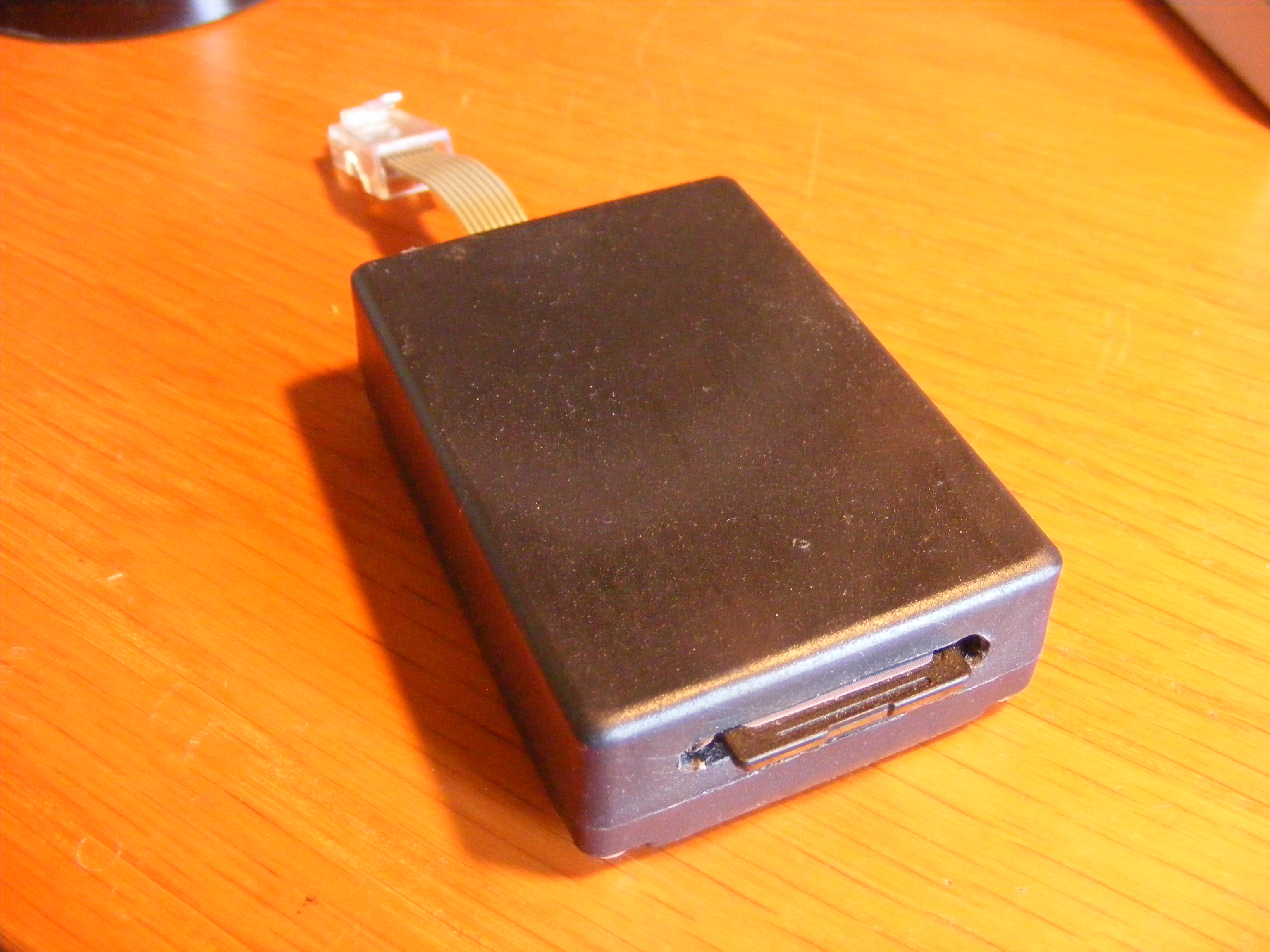
The SD-standard is a semi-open standard. You can join
an SD-society, but it probably costs a couple of milions.
If you are not a member, there is a rough public spec. It is
actually not bad, but some questions remain unanswered.
There is useful information on this site:
elm-chan.org/docs/mmc/mmc_e.html.
There are two protocols for the SD-card, one called
SD-bus, and the other is SPI. Amateurs probably prefer
SPI; the SD-bus seems unnecessarily complicated. A special
issue is the so called CRC, Cyclic Redundancy Check.
With CRC, you are supposed to add a so called CRC-code
to the message you send. If there is any error in the
transmission of the message or of the code, the receiver
is able to detect this. CRC-codes are generated by a
very interesting algorithm, but with the time I have spent
on it, I haven't been able to penetrate it, so I can't
compute CRC-codes in real time. Fortunately there is a
web-page, that can compute CRC-codes off-line:
ghsi.de/CRC
Fortunately, the CRC-checking is disabled in SPI-mode,
though not quite.
So, we all want to use the SPI protocol. However, SanDisk,
which is probably the major supplier of SD-cards, have
abandoned the SPI protocol for their SD-cards, which means
that they break the specification of their own society.
I've tried Verbatim-cards and Kingston-cards, and they
work.
SD-cards come in a newer standard called SDHC (High Capacity),
and I thought it would be wise to adapt to this new standard,
as it might be difficult to find regular SD-cards in the
future, specially if I have to keep away from SanDisk.
The point is this: You adress an SD-card with a 32 bit
adress. That's good for adressing memories up to 4GB
(232 is approximately 4 bilions). But SDHC cards
are bigger than that. So instead of letting the adress be
the adress of a single byte, you let it be the adress of
a block of 512 bytes. When you read and write, you can
only read and write full blocks. When you read you can find
your interesting
byte somewhere in that heap of data. This is in a way good.
When you write, you always write a whole block, which
you can do without problems. Block writing automatically
opens the memory for writing. And you read almost the
same way as you write.
But there is a job for you in this context. You have to
tell the card, that you have understood, that it is an
SDHC-card. For some odd reason you have to send this message
with a correct CRC-code. But this is a static message,
so the CRC-code is static, and you can find it on that
web page.
The cards are controlled by numbered control commands.
The message starts with binary 01, and then follow
6 + 8 bits of command. Then follow three bytes of
parameters associated with the command, then the CRC code
and a single bit 1. In the sequel I give the command
number as including the 1 in the second bit. That means
that all commands are greater than $40 (in the way that
hexadecimal words are written in the Propeller world.)
Card initalization
Now, let's take it from the beginning. The SD-card needs
clock cycles to get through its own initialization procedure.
It seems that the card computer doesn't have a clock.
A simple way to achieve this is to send 8 bit data with
the SPI protocol. I send 20 such bytes, which is probably
more than enough.
Now, the card wakes up in SD-mode. It is comfortable
but strange, that we can still send an SPI-message to it.
That message is $40 (hexadecimal 40), with
a zero argument. And it has to have a correct CRC-code.
But many amateurs have found out that this CRC code.
is $95. (formally it is $47, but after you've squeezed in
that final 1, the last byte is $95.) This command puts the card in idle mode, but
it also tells the card, that we will talk to it in SPI-mode
Then we must give the message "I know, that you are an
SDHC card". The command is $48, but this is a kind of a
group command, so it needs a parameter $1AA. The CRC-code
is $43.
Then we need to leave the idle mode. It is a command $69
but it belongs to an expanded group of commands (so called
app-commands) so we have to send the command $77 before
it. The command $69 has a parameter which is 1 in the
thirtieth bit.
The card always sends a response to the commands. There
are different categories of responses, but this is the simplest
of them. In it, the last bit represents that the card is still
in idle mode. So we will keep sending these commands until
the response is 0. With that, the card is initialized.
Once you have downloaded the software, take a look to
see if it fits with this description.
Writing the card
To begin with, writing is simple. We just write the
data to our own writebuffer in the Propeller.
We build the writebuffer in longwords,
and there are 128 longwords in the buffer (=512 bytes). We
strip off the last 7 bits of the adress as in-buffer-adress.
In every such write operation we increment the adress by
1. Initially, we have set the adress through a set adress
function.
But when the in-buffer-adress reaches 127, we have to do
more. We have to write the data out to the card itself.
The command for this is $58, and the parameter is the
block adress, which is the adress except the 7 last bits.
We can then put anything as CRC code. This command should
then be followed by a so called token, which in this case
is $FE. Then we send the data byte by byte, so we have
to extract these bytes from the longwords in the writebuffer.
Then we send two arbitrary numbers as CRC for this whole
data packet (this is supposed to be a longer CRC of 16
bits, while the CRC codes mentioned before are 7 bits long),
and then we wait for a response from the card.
The card now has all the data, but it takes a while to
actually write them to the card. In the meanwhile, the
card will send a busy signal.
Reading from the card.
The read system tries to find the data in the read
buffer first. This supposes that no one has written new
data to the card since the buffer was downloaded from the
card. This fits with the assumption that we don't write
and read the card in anarchy.
For this, the system has a current block number
(called rbl), which
is the number of the block most recently downloaded.
From the read adress, the block number can be extracted
as the bit pattern except the last 7 bits. If this block
number equals the current block number, the data can
immediately be read from the buffer.
If not so, we have to download a new buffer from the card.
This is done with the command $51 with the block adress
as argument. Then we wait for a response from the memory,
and then we clock in the data by using the spi.exch
command. We also use it to clock in two bytes of
CRC-code for the package from the card.
Now the buffer is updated, so we can read the desired
datum from the buffer.
The object file
The SD-card is handled from an object called sdh.mpo
("h" for "H" in SDHC). The functions there are called in
following way:
( dipin , dopin , clkpin , cepin , )sd.init
( dipin , dopin , clkpin , cepin , )sd.connect
( adress )sd.setadress
( data )sd.write
)sd.readbyte ->data
( longadress )sd.read ->data
Except for these functions, there are some functions
used internally. sd.write and sd.readbyte
write and read sequentially from the adress set in
sd.setadress. sd.read requires an adress
to read from in each call.
I have been using a breakout board for an SD-card holder.
It is marked with pin designations according to the
SD-bus standard, so here is a translation to SDI-designations.
Note that SO means "out of the card" so it is for
traffic into the computer. The opposite holds for SI.
- d2 is unused but it should be pulled up Vcc
with a resistor of some 10 kOhms
- d3 is chip select (cs or ce with negative logic)
- cmd is SI
- cd is to be grounded
- clk is sck, the clock signal
- vcc is supply voltage
- gnd is ground
- d0 is SO
- d1 is unused, but it should be pulled up to Vcc
with a resistor of a couple of 10 kOhms
- wp is unused
EEProm
The standard program memory that Parallax uses for the
Propeller is called 24LC256, but if you can find it, it
pays to buy a 24LC512 instead. You get twice as much
capacity for almost the same price. 512 means 512 kbits,
organised as 64 kBytes. (we will mention a version
with even more capacity here)
But you can do more than that. The chips have three pins
called adress pins. Parallax advises you to ground all
these pins, to make for the adress 0. In fact you don't
need to. The pins have a pull down circuit, so they "ground
themselves". But if you add another chip, you can give
it another adress, by pulling some adress pins high. Then,
alltogether, you can have 8 different 24LC512:s with unique
adresses. So, the maximum capacity of such a system is
512 kBytes or one half Meg. We call these subadresses,
set by the adress pins, chipadresses.
These memories are pretty straight forward
I2C-components. In the I2C world, each
circuit type has its own device adress, though these
device adresses can hardly be distributed in such an orderly
fashion as IP-adresses or Bluetooth adresses. Anyway,
these memories have the device adress $A0. But then
the above mentioned chipadresses fill the three bits after
the 'A'. The final bit is a read/write bit; 0 for writing.
Then the chip with the chipadress 3 is adressed for writing
with $A6.
The protocol is then as follows:
If you want to write to the chip with chipadress 3
(as an example), you start with the start pattern.
and continue with the code $A6. Now the appropriate chip
will listen, and all others will go to sleep. Next you
send the adress within the memory, which takes up
16 bits for 64kBytes, so you have to send this adress
in two bytes (the most significant first). Then you can
just send your data in bytes. After each byte, you have
to wait for an acknowledge signal from the memory.
(it's no really just waiting. You're the host, so you
have to send the clockpulse to get any response.)
Finally you send a stop pattern.
If you want to read from the memory, you start the same
way, sending device adress, and the adress within the
memory. But then you have to send a new start pattern, and
then again the device adress but with a read bit. So in
the example, the code to send is $A7. Then the component
will send you the data byte by byte, encouraged by the
acknowledge patterns you send. You stop the traffic at
any time by sending a stop pattern instead of an
acknowledge pattern.
These memories behave pretty much as RAM-memories in the
sense that the time it takes to read and write, is
independent of the adress. But they are slower to write
than to read. When you have sent data for writing to the
memory, they have just been buffered so far, so you have
to wait some extra time, before they are acutally written.
The object file eeprom.mpo contains functions for
handling the EEPROM. You can initialize the memory system,
and then you can set the chipadress (called chipcode),
to adress a particular
chip. There is no particular support for writing over
the boundaries of the chips. Then you can set a start adress
for reading and writing, and this adress is then incremented,
when you read and write. You can read and write bytes
and longwords. But you can also move chunks of data between
an array called ee and the EEPROM. If you use that,
you have to declare ee as a global variable. Here's
how the functions are called:
( clockpin , datapin , )ee.init
( chipadress )ee.setchip
( adress )ee.setadress
)ee.readbyte
)ee.readlong
( data )ee.writebyte
( data )ee.writelong
( from , to , n , )ee.read
( pageadress )writepage
from is the adress in memory from which reading
starts. to is the adress in the array ee
where the first data are written. n bytes of data
are transferred. The concept of page is an area
of 64 bytes in the memory. pageadress is a numbering
of the pages, which is made by stripping off the 6 last
bits of the normal adress. writepage writes
the 64 first data in the array ee to the page
in memory.
You can upload data for a program to the EEPROM. Then
you need an upload program, using the write functions.
And then the actual program has to use the read functions.
On the other hand you can use the EEPROM to logg data with
the write functions. Then you have to start a download
program using the read functions, to get you data to,
say, a PC.
Flash memory
The flash memory I have used is from SST and is called
SST25VF032B. It has a capacity of 4 MBytes.
It comes in an 8 pin surfacemount package,
which is not all that hard to work with. It's a pretty
straightforward application of the SPI protocoll.
Two things are a little more difficult. One of them is
the write protection mechanism. It is nice of SST to be
careful about my data, but after all, I would like to
write something at some time. So we have
to break open the write protection mechanism. First there
is a WP-protection pin, that has to be high. In that
situtation, it is in principle possible to write to the
status register, that controls the write protection. You
can do that with a Write Status Register command WRSR.
But before that, you have to enable the writing of the
statusregister with an Enable Write Status Register
command. But that command is not allowed, unless a
Write Enable command has been sent before it. For all
these instructions you have to handle the chip select bit,
that belongs to the SPI protocol. When you have found
all this out, it is not terribly complicated, but after
you've read the spec, you couldn't feel sure about it.
It is about trying. In the object file Flash.mpo
there is a function called fl.open which does all
this. It involves a call to fl.wren, which is used
in many places.
The other difficult thing, is that this is a flash memory,
and you don't write to flash memories just like that. You
have to erase it first. You can erase the memory in blocks
of 1024 longwords (there are 1024 of these). When the block
is erased, all bits are just 1. While writing, you can
change any bit to 0. If you try to write to the same cell
again, new bits are changed to 0, but nothing ever gets 1
without erasing. There is also a command for erasing the
whole memory. It is the fastest way to erase the memory, but
you erase all your data. All this, of course, calls for some
planning.
The protocol is like this. You send a command number, and
then the adress, split to 3 bytes (which would be good
for 16MBytes, but 2 bytes of adress is insufficient for
1 MByte). And then you send your data, or receive your
data. You terminate this traffic by pulling the chip
enable bit high.
Here are the command codes used:
- $02, for writing to the memory
- $03, for reading from the memory
- $06, for enabling writing to the memory and
its status register
- $50. for enabling writing to the status
register
- $01, for actually writing to the status
register
- $05, for reading the status register
- $20, for erasing a block
- $60, for erasing the whole chip
And here are the functions, and the way they are called:
( dipin , dopin , clkpin , chipenablepin , )fl.init
( byteadress )fl.bread ->byte
( longadress )fl.read ->longword
( longadress )fl.erase
)fl.chiperase
( byte , byteadress , )fl.bwrite
( longword , longwordadress , )fl.write
)fl.open
You can see, that we look at the memory in two different
ways, either as a memory of bytes, or as a memory of
longwords (32 bits). When we regard it as a memory of
longwords, we adress it accordingly, i.e. with a longword
adress. The next longword in memory then has adress + 1,
even though it is 4 bytes up. In fl.erase,
longadress is any
longword adress. The system itself will erase the whole
block, that contains that adress.
If you look at the code for fl.write, you can see
that it uses fl.bwrite four times, which is far
from efficient, so there is room for improvement (You can
send all four bytes of a longword in a single write
command).
You can also see that writing a byte takes a little more
than 15 microseconds. But to erase a block takes 40
milliseconds, and this will effect the speed of writing
much more. In my applications, the data rate has been
lower than one data per 40ms, so then there is no problem,
but if this is not the case, you have to buffer data, and
erase the next block while buffering data.
A File System
I have made a file system for the flash memory.
I tried to do it for the SD-card, but I haven't been
successfull yet.
The key issue for a file system is that you should be able
to erase files. After you've done that, you have some space
left. If you try to squeeze in a bigger file there, you
have to give up. If you have a smaller file, you will get
an even smaller space left. As you write and erase, the
memory space will be more and more like a Swiss cheese.
The trick to handle this, is called fragmentation.
You divide all files in equally sized fragments. When you
have erased your file, a number of fragment spaces will
be free to fill with fragments from your new file. If the
new file is smaller, then some fragment spaces will still
be free for future files.
The fragments are kept together by links. So when a
fragment space has been filled, you have to find a new
fragment space elsewhere, and then you write a link to
that fragment space, last in your current fragment. When
reading the file, we have to follow these links through
the file.
In operating systems like Windows, there uses to be
a program for defragmentation. This might seem as
a cure for the fragmentation disease. But fragmentation
is not a disease. It is a necessary part of a file
system. But - for physical memory devices like hard disks,
it's better if the fragments are not physically too far
away from one another. To move from one part of a hard disk
to another, far away, may take maybe a millisecond. It doesn't
sound like much, but if you have to do that thousands of
times, when reading a big file, it gives you a very noticeable
delay. Hence, defragmentation is about moving the fragments
of a single file as close to one another as possible on the
surface of a hard disk.
You may think that a file system is much about creating a
hierarchy of files with so called directories. But all this
is just a name issue. Say that you have a directory
c:\propeller\mps and that you have a file there called
flash.mpo. Then the actual real name of that
file is c:\propeller\mps\flash.mpo. Now, if the
systems thinks you are "in the directory"
c:\propeller\mpo (and informs you about that with
e.g. a prompt), then the system will automatically add
c:\propeller\mps\ to the filename you write. So
if you write the filename flash.mpo, you will
automatically get the right filename. This gives you the
impression that the file flash.mpo is in
the directory c:\propeller\mps\. In fact, all
files are all over the place on the disk, specially as they
are fragmented.
My file system is much simpler, when it comes to names. A
file name is only 3 bytes long, i.e. three characters. It
doesn't allow for any system of directories, but it is
enough for my purposes. The fragments of the files coincide
with the blocks of the flash memory, i.e. they are
1024 long words. That is really a little too much, if you
have many small files.
Then there is a file catalog,
which takes up the 64 first longwords of memory block 0.
Each file here is represented with its name in the first
three bytes of the longword. The last byte contains the
block number, where the file begins. This allows us to
let the files begin in the first 255 blocks. But then
the files can continue in blocks with higher block numbers.
After the file catalog, in block 0, follows an account
for which blocks are busy in the memory. Each block has
a bit for this. So we need 1024 bits, which takes up 32
longwords. Block 0 is always marked as busy, as it should
contain the file catalog - and this busy accounting
structure. The busy accounting structure is called
occu.
In each block, words 0 to 1022 are sequentially filled with
data, but the last word is the link to the next block.
When we try to write data there, we should observe that
this place is reserved for a link. Then we should find
a new block, by inspecting occu. We prefer to look
for free blocks above number 255, as the lower numbers are
good to have as first block in each file. We don't need
to erase the new block, because we assume that this is done
either initially, or when we delete a file. After we
have chosen a new block, we just write its number
in cell 1023, and then we move to the new block,
and write our datum there.
The file catalog and occu belong to a block in
the memory. Such a block can not be handled easily, as
we cannot change data in the block without erasing the
entire block. Due to this, we have to create a mirror
image in the Propeller of this block. We keep the two
mirror images updated by writing mutually, whenever
anything changes.
There is a danger in this for battery driven equipment.
The computer will stop working when the battery falls
under a certain level. This is likely to happen when
a block erase of the memory occurs, as a block erase
consumes pretty much current. If so, the computer is lost
in a precious moment, when it should restore the file
catalog after it has just been erased. I've seen this
happen. The file catalog is gone, but with some detective
work, I can still read the files. But with the file
catalog gone, it is impossible to manage further writing
to the memory.
Of course I can't be
quite sure about the causes of this loss of the catalog.
The state of an individual file is just, except for the
data we have written into the memory, a pointer to where
we stand, and are ready to read or write. (In this system,
a file is either being written or being read, never both.)
The pointer is practically three variables. One is
block, which is the block where we stand, and the
second is pos, which is where we stand in position
within the current block. The third variable is called
bit, and tells us which bit we are currently
reading or writing. It would allow us to write and
read the memory bit by bit, but right now it is
only used to read the memory byte by byte. But
normally, the file system regards the files as
files of longwords. (Slightly unconventional, but
I prefer to view the Propeller as a longword machine,
and then it is practical to regard the memory as the
same.)
The file system is built according to the principle of
a class, and instances of a class. This means that the
variables that belong to the file, i.e. block,
pos and bits are arrays. The index to the arrays is the
last argument to every function. (This is what was called
unit numbers in Fortran). So you can open a file with
index 3, and write data to it with that index. At the same
time, you can have another file with number 2, which is
completely independent.
Files are files of longwords. The file system, as mentioned,
is kept in the flash memory. Thus, the file system serves
as an interface to the flash memory, where the flash
memory is completely invisible to the user.
Here's how the functions at file.mpo are called.
The file index (Fortran unit number) is called k:
( dipin , dopin, clkpin , cepin , )f.init
( dipin , dopin, clkpin , cepin , )f.connect
)f.grandreset
( name , k , )f.open
( name , k , )f.new
( data , k , )f.write
( adressofstring , k , )f.swrite
( k )f.close
)f.eof
( k )f.read ->data
( k )f.readbyte ->databyte
( name )f.delete
( c1 , c2 , c3 , )f.name ->name
f.init sets up the communication with the memory
and f.connect reestablishes this communication, if
we have changed process code in a cog. f.grandreset
resets the whole file catalog, and erases the whole
memory. In the PC-world this is something you do
"once in a lifetime" for a computer, but for these smaller
devices, I guess you do it more often. A Propeller is not
a part of an archive. f.open opens an existing file
for reading. f.new opens a brand new file for writing.
f.swrite writes a null terminated string to the
memory. The format is the usual one, that each character
takes up a full longword. f.close closes a file
by writing an "end of file"-symbol at the current pointer
position. The symbol is "e","o"."f",0 packed into a
longword. For comparison, you can retrieve that symbol
with the funcion f.eof. f.readbyte reads
a single byte from the file, and then moves the pointer
one byte forward (on fourth of a longword) by manipulating
the bit variable. In the f.delete function,
you refer to the file by name, and not by unit
number k. Finally f.name is a "name factory".
It packs the three characters c1, c2, and c3 in the
three least significant bytes in name. This is the
form names have, when you call f.open and f.new.
When you use this file system, you have to make the following
declarations of global variables:
block[5]
pos[5]
bit[5]
cat[64]
occ[32]
A File System for the EEPROM
Lately, the EEPROMs as described above have come in a
version with 1024 kbits, which could maybe be enough
for some applications. Problems I have had with a
GPS logging system, encouraged me
to make a try to use these memories for GPS-logging.
In that application, I store three longwords per seconds.
That is 12 bytes, and the memory has a capacity of
128 kBytes, so I could store 10000 samples, which is
well over 2 hours. If I would like more, I could change
to sampling every 2 seconds.
First a note about these components. The 1024kbits is
organized as 128 kbytes. To adress that space requires
17 bits. But in the protocol to control these components
over I2C, we only send 16 bits. Rather than
changing this, the manufacturer has chosen to send the
17th bit in the device adress. That device adress consists
of the device code (hexadecimal A) + three free bits + a
read/write bit. The three free bits were supposed to
to match values set to three input pins on the chip.
Now, the first of these bits is instead used for the
17th adress bit. Previously we had 3 bits, so that we
could build a battery of 8 chips. Now, with only 2 bits
left, we can only build a battery of 4 chips. The chip
still has three adressing pins, but now we can only use
two of them. For some reason, it has been decided that
the third bit has to be connected to the voltage supply
line. If you forget that, the memory won't work. This
is described in the data sheet.
The EEPROMS have the advantage over the Flash memories
I've used, that I can write to individual adresses.
That means that I don't need any mirror areas in the
computer. As I had some problems with that (see
here), I decided to build
a file system for the EEPROMs, as an alternative, and that
is now what I use in the GPS logg application.
Writing to individual adresses is fine, but it comes at
a cost. Firstly, writing an individual byte takes as
long time as to write a whole page of bytes, and this
is about 4ms. If you write individual bytes, this is
the average time it takes. If you could buffer your data,
and write a whole page at once, that again would take
4ms, so your average write time would be much shorter.
But the maximum write time would still be 4ms. But
there is more to it than that. EEPROMs, which are in fact
flash memories, wear out after a milion writes or so.
When you write individual bytes, the memory chip still
has to write the whole page. So the number of writes
is much bigger giving the EEPROM a shorter life. But
for the applications I have in mind, I don't think this
matters too much.
Then, another thought has caught me. In my other file
systems I had a global array of pointers to point at current
block and current position. This was fairly costly, so I
decided to have only single pointers, and then I could
make them local, by letting them be field variables in
my file system object. That would mean that I could
only hold one file open at a time. But this is not quite
true. If I manipulate files in separate processes, I
can handle them individually. The pointers are local
variables, and so there are instances of them for each
process (cog).
The end of this, is that there are no global variables
at all. The file catalog and occ are in the EEPROM only,
and the pointers are local field variables.
The EEPROM has pages of 128 bytes (the smaller EEPROMs have
pages of 64 bytes). I like to see the
memory as a memory of longwords, and then the pages
are 32 longwords. The first page, Page 0, is used for the file
catalog. With that I can maintain 32 files. The
next page is used for the correspondent of occ, i.e.
as an account for which pages are occupied by files.
There are altogether 1024 pages, and these can be
represented by the 1024 bits of the 32 longwords in
page 1. Page 2 is reserved for a single filename for
the GPS application, so actual data are stored from
the Page 3 and up.
Then, files are stored in "fragments" filling up one
page each. In the file catalog, each entry consists of
a three byte (character) file name, and then a pointer
to the first page. Then, when a page is full, a new free
page is sought for, and a link to that new page is
written into the last word of the page. The EEPROM, unlike
the other flash memory, is never erased completely, so
to be sure, whenever a new page is reserved for use,
a pointer 0 is written to its last word. This 0 will
be overwritten by a new link, when the page is full.
Specially, in the GPS applicatione, there is never time
to write an end-of-file-symbol, because logging ends
when power goes away, and then it is too late to write
the end-of-file-symbol. Then, the end of the file is noted
when a 0-link to the next fragment appears.
To read the files, one just follows the links
through the fragments, until an end-of-file-symbol is
encountered, or until a 0-link is detected. In the latter
case, we have usually read a little too much, but it is
not always a problem. When deleting a file, we have to
follow the links, and set the corresponding bits in
the words in page one back to zero again. And we erase
the entry in the file catalog. But no actual erasing of
data is necessary.
Here are the functions of the object in fileE.mpo,
where the 'E' of course symbolizes the EEPROM:
- )f.grandreset resets the file catalog and
the "occ array", but else, the memory is not erased.
But the file system will appear to the user as
empty and free to use.
- ( clockpin , datapin , )f.init initializes
the file system by initializing the communication
to the EEPROM chip, but it leaves the content
of the file system intact. The pin numbers are
the pin numbers to the EEPROM chip. You can use
the same pin numbers as the Propellers standard
EEPROM, but you have to give you chip another
hard wired adress than 0.
- ( name )f.open opens an existing file
for reading. name has the three characters
of the file name in ASCII code placed in the
three least significant bits in the word.
- ( block )f.openfrom can be used for detective
work, when the file catalog has disappeared. I
don't think it will be necessary to use now.
The function opens the file that starts att
block 'block'.
- ( name )f.new opens a new file for
writing. The name is reprsented as for f.open.
- ( data )f.write writes a longword at
the end of the file.
- ( adress )f.swrite writes a string to
the file. Each character takes up a full longword.
Writing ends when the function encounters a
null character (null terminated string). The
string should be a local variable, and its
adress is 'adress'
- )f.close writes an end-of-file-symbol
to the file.
- )f.eof is a utility function that delivers
the end-of-file-symbol to someone who wants to
use it.
- )f.read ->data reads a longword from
the file.
- ( name )f.delete deletes a file with
the given name, as described above
- ( "x" , "y" , "z" )f.name constructs a
the filename "xyz".
The remaining functions are for internal use. There is no
)f.connect function as such a function couldn't be smaller
than the )f.init function. It wouldn't be necessary to
initialize the file system in its own process.
The file fileE.mpo uses functions from the object file
eepromm.mpo, which interfaces to the bigger EEPROM
24LC1025.
Human Interface Devices
Potentiometers can be good as human interface devices.
Their outputs can easily be connected to A/D converters,
and those are controlled by functions in the standard
object file std.mpo. Some other interface devices
require a little more.
Keyboard
The object file key.mpo contains a relatively simple
collection of functions for handling a standard
ps2 keyboard developed for the PC many years ago.
The ps2 communication was a serial communication protocol
not quite unlike the SPI protocol.
The communication is handled
by two function kb.rec and kb.send. Unlike
SPI, the communication is clocked by the keyboard, so
as a receiving computer, you have to be alert to catch
when the operator hits a key.
The object normally only receives data from
the keyboard, but there is a historical circumstance, that
forces us also to send to the keyboard. The creators of
ps2 decided that the PC and the keyboard should synchronize
the following way. The keyboard would repeatedly send a
character, but with the wrong parity. Synchronization would
be established when the PC complained about this. So we
have to send such a complaint message.
The user has to call the function key.init. He
also has to declare two global variables key and
keyp. Keys are scanned with key.scan. This
is the function that has to be alert at all times.
Thus, it has to have its own process.
The keycode for the key pressed the latest,
will be deposited in the variable key.
Keycodes are seemingly arbitrary numbers assigned at the dawn
of computing, but they do reflect the position the key has
on a standard English keyboard.
The A-key has its number, as well as the shift key. The
latter would enable us to distinguish 'a' from 'A', but
we don't care about that here. When a key is released,
key will assume a value called 'break'.
Now, we can call the function key.ascii. It will
translate the key code to the corresponding ascii code
and return that.
As long as we keep a key pressed, a call to key.ascii
will return the ascii code of the key. When the key is
released, the function key.ascii will return 0,
which is the ascii code for the null character.
Right now, I have a numerical keyboard, rather than a full
size keyboard, as it is handier. Then, to produce figures,
I use the keycodes, that the numeric keys have on the
so called numpad part of the keyboard.
So the functions to call are the following:
)key.init
)key.scan
)key.ascii
Touchscreen
As an amateur, you can buy a type of touchscreen formerly
used by Nintendo. They are cheap and simple to use, but
of course they don't compare with modern touchscreens used
in smartphones. They are still usefull, but you need a little
stylus to handle them; they don't work well with your
fingers.
They are resistive devices consisting of two conductive
sheets, which can be brought to touch one another, when you
press them. One of the sheets has two horizontal metal bars
up and down. The other has two vertical bars right and left.
Say that you apply high voltage (3.3v) to the upper bar,
and low voltage (0v) to the lower bar. This will create
a potential field that varies linearly over the sheet.
Then you connect say the left bar to an
A/D converter, and let the right bar float.
The high impedance of the A/D input means that there is no
current through the second sheet, so the voltage over
the second sheet will be constant. When the two sheets
touch one another, that voltage will be the voltage at the
contact point. In this way, we get a measure of the
y coordinate of the point of touch. To get the x coordinate,
we just have to shift the roles of the upper an lower sheet.
To put this under program control, we connect all four
bars each to its own Propeller pin. For the active sheet,
we make them output pins, and give 1 and 0 to them. For
the passive sheet, we set the pins as input pins. Then we
connect two of these pins to input channels of the
A/D-converter.
We also have to detect the situation that the touchscreen
isn't touched at all. For this we connect one of the
A/D channels to 5 volts through a reasonably big resistor
(10 kohms should be good). This resistor will pull out
the voltage to values, where it couldn't be if there were
contact.
Here are the functions of the object file touch.mpo,
and how they are called:
( chy , piny1 , piny2 , chx , pinx1 , pinx2 , )touch.init
)touch.get 0>x 1>y 2>valid
)touch.get )touch.censor 0>x 1>y 2>valid
touch.get delivers its result in the three
variables arg0, arg1 and arg3, and they can be retrieved
with the instructions shown. If valid is false (0),
then the screen is not touched, so you should not use
the values. The last line indicates the use of a function
touch.censor. With that code, x and y will not
be updated if there is a big jump in values.
You can also download a program draw.mps (see under
MPS Objects below) that lets you draw sketches on the
touchscreen, that appear on the graphical display. Move
the stylus out towards the right edge to erase.
Here's the setup with the touch sensor and the display,
and the greek characters alpha, beta and gamma drawn.
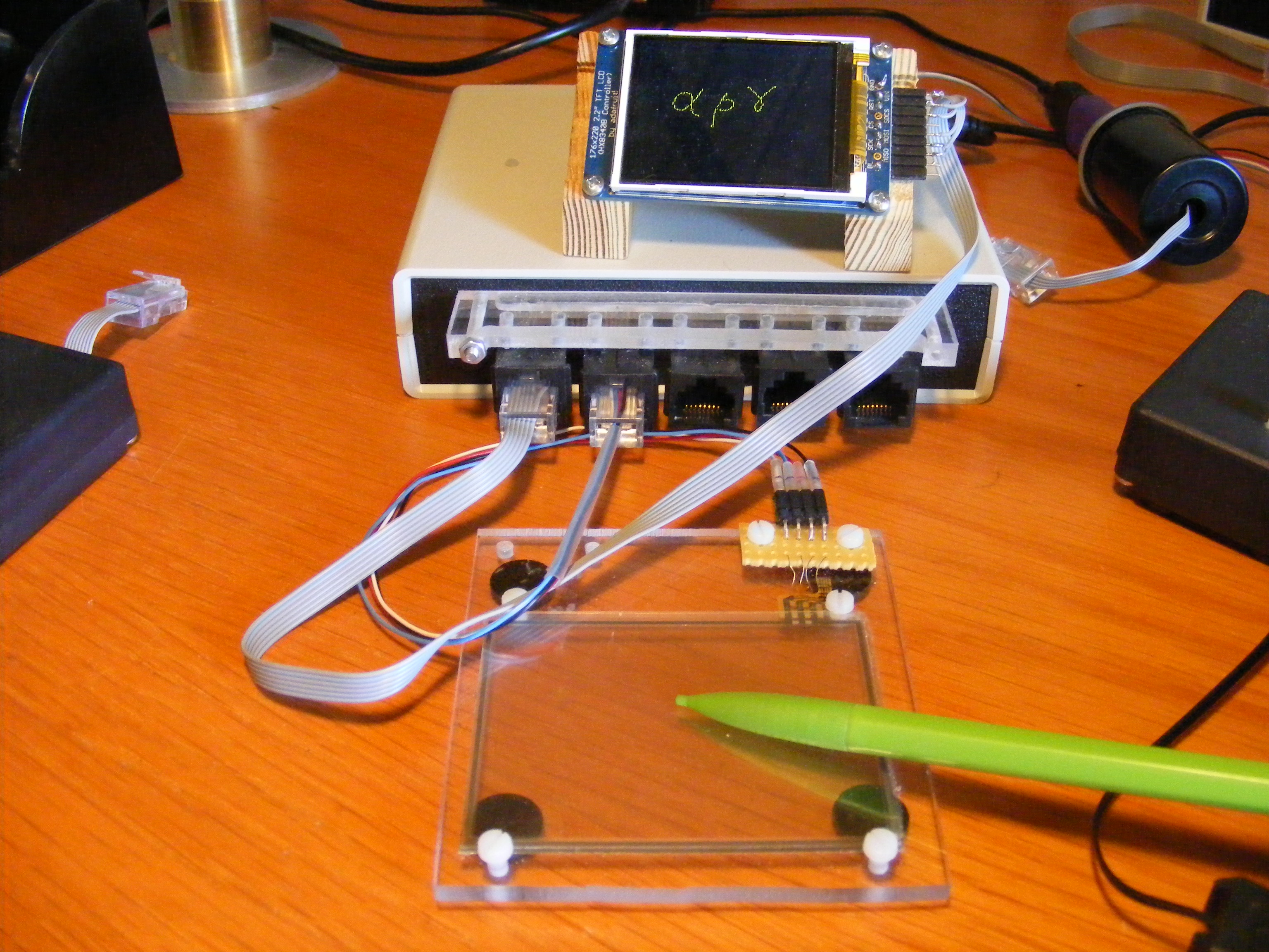
And here's the result (There is an interference pattern
called Moirée pattern, when you photograph a display with
a digital camera):
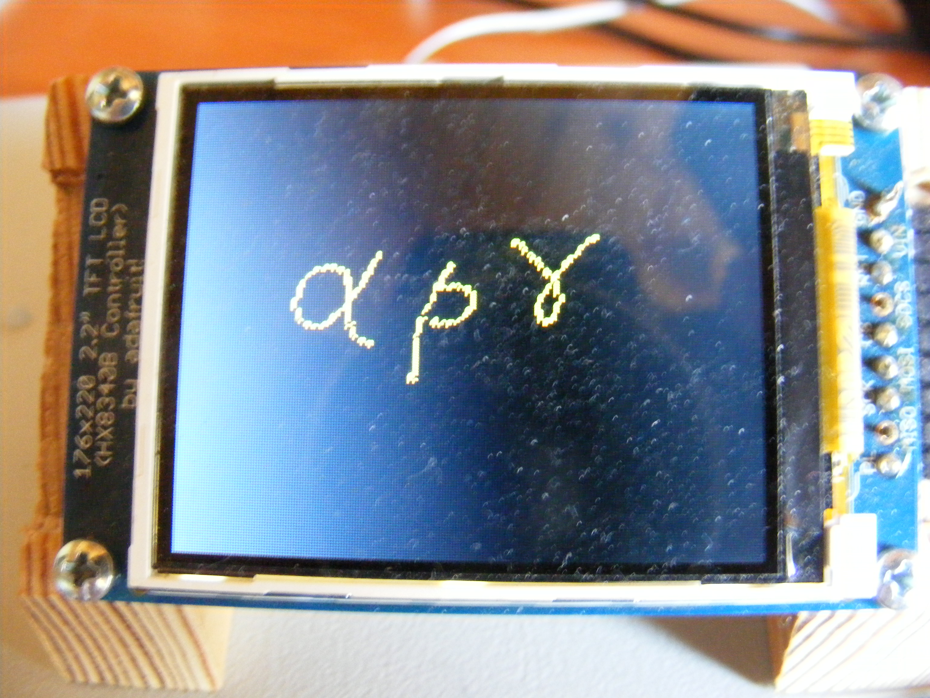
You can mount this touchsensor on top of a graphical display.
That's when the thing really deserves the name
"touchscreen". But these touch sensors are sold
separately, and they seldom have the same format as
a display, and if you mount them together, there is an
unavoidable distance between the two, that creates a
parallax. So I never did that. Otherwise, the idea would
be that you would draw icons on the screen, and point at
them with the touch sensor. I have preferred to draw
the icons on a slip of paper, and put that under the
touch sensor. It's not so dynamic, but it gives you a
multi mode mode control.
Accelerometer
An accelerometer is not in itself a human interface
device. It's a sensor. But you can use it to build a
joystick.
Those who sell accelerometers use to say that they can
be used to measure two things: acceleration and tilt.
In fact, they can measure none of them, but just a
confusing mixture of them. The deeper reason for this
is that acceleration and gravity are indistinguishable,
which was the basis for Einstein's foundation of the
General Theory of Relativity.
But this means, that if we don't move the accelerometer
with too much vigour, we can sense its tilt angle.
Then I've built the accelerometer into a plasic
tube with a heavy brassfoot, that makes it stand up:
The accelerometer is padded in there between two
pieces of plastic foam.
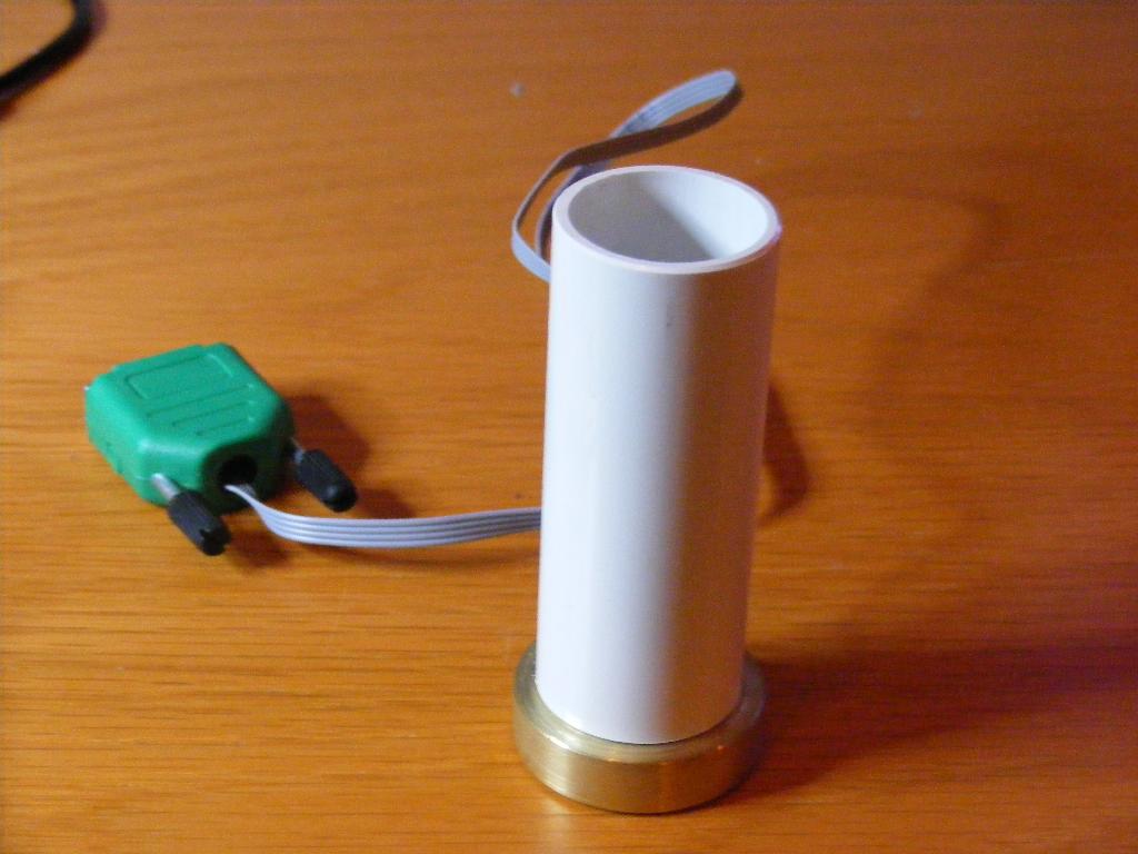
If I grab it and tilt it, I can read off the tilt
position, and use that to control a program.
But you can also mount the accelerometer on a vehicle,
and use it to measure acceleration. But remember: The
signal is always disturbed when the sensor is tilted.
The code is made for an acceleration sensor called
Memsic 2125, which delivers pulses, whose widths vary
with acceleration, and with a width of 5 ms for no
acceleration. These accelerometers are sold by Parallax.
Electrokit in Sweden sells an accelerometer called
DE-ACCM2G. It has direct analog outputs for the
acceleration, so with an A/D converter, they are easy to
use. It has a range of +-2g, which is more than you need
for the joystick application, but there is a +-6g version
also. SparkFun sells, among others, an accelerometer from
Analog Devices called ADXL335, which is probably of very
high quality. It is a three axis accelerometer, while the
others mentioned ar 2 axis. The outputs are analog (I think),
The object acc.mpo, which works for the accelerometers
from Parallax, has functions to be called as follows:
( xpin , ypin , )acc.init
)acc.get 0>ax 1>ay
There is a third function for scaling, but it's used
internally. acc.get delivers the results in
arg0 and arg1, but they can be retrieved with instructions
shown. The output range is 0..4096 with 2048 representing
zero acceleration.
Odometry
Odometry comes from a Greek word for "way" or "road",
and it is the art of determining travelled distance.
To do it we have a striped strip and two optical sensors.
We can put that strip around a wheel of a robot, to measure
its travelled distance, or we can glue the strip on the
road itself, that we travel along. Here's how it works:
We have two pictures of a strip and two optical sensors
(the circles) in both pictures. The optical sensors are
reflex detectors, which consist of a light source (IR-LED)
and a light sensitive component. The strips move as
indicated. In both these cases, the right hand detector
switches from white to gray, which indicates a motion. But
which motion is it, the upper or lower case? We can tell
by looking at the left hand sensor. In the upper case
it is white, in the lower it is grey. So now we can
detect a motion "with sign", and we can accumulate the
incremental motions to a distance travelled.
The Odo object odo.mpo handles two strips and two sets
of optical sensors, to determine movements in the plane.
The functions are called as follows:
( chx1 , chx2 , chy1 , chy2 , )odo.init
)odo.get 0>xo 1>yo
chx1 etc. are the analog channels to which we have
connected the optical sensors. The result from odo.get
is delivered in arg0 and arg1. The result is the total
travelled distance since initialization.
Color Object
This is a very simple object, that handles a three color
RGB-LED. The use is maybe most for debugging. You can
get a certain color, when you come to a specific place
in your program, or when a variable has assumed a specific
value. To make it simple to use, the object has no
init function. You call the only function in the object
col.mpo like this:
( number )col.show
The color emitted is controlled by number as follows:
- 0: red
- 1: yellow
- 2: green
- 3: cyan
- 4: blue
- 5: magenta
- 6: white
- 7: black
- 8: yellow (again)
The current program assumes that the LED pins are
connected to pins 5,6 and 7. The LED is an array of
three diodes connected with the cathodes common. It
is connected like this:
With the extra silicon diode at the green LED, we
get a reasonable balance between the colors. The
supply voltage of 5 volts is not critical, but 3.3 volts
may be too low.
It's nice if you can dim the LED by letting it shine
through a piece of white plastic. I let it shine through a
nylon screw threaded into the computer box. With the diode
in place, you can make other stuff, like mixing colors
using pwm technique.
MPS Objects
Here are download opportunities for object files already
mentioned:
A way to get these files is as follows. Click one of the
links above. Then hit ctrl/A to select the full text.
Then hit ctrl/C to copy the text to the computer paste buffer.
Then open e.g. Windows Notepad, and drop the text into
it by hitting ctrl/V.
Complex Number Object
Here's an object file for objects that are so called
complex numbers.
In higher mathematics, a complex number is defined
as a pair, (x,y), of real numbers x and y together
with the following addition and multiplication rules:
(x1,y1)+(x2,y2)
= (x1+x2,y1+y2)
(x1,y1)*(x2,y2)
= (x1*x2 - y1*y2,
,x1*y2 + y1*x2)
Then, there is the style, to write (x,y) as x+i·y. We think
of x + i·0 as just the real number x. We call 0 + i·y just
i·y, and 0 + i·1 just i. Now, if we take (0,1)*(0.1) alias
i·i alias i2 and use the above multiplication
rule, we find that i2 = -1.
This has lead people to name i "the square root of minus one".
And it is, but only if we introduce these very special
pairs of numbers, called complex numbers, and with this
very special mulitiplication rule, and only if we consider
the pair (-1,0) as the same thing as the real number -1.
If we accept that i2 = -1, and write our pairs
as x + i·y, and expand the product (x1 + i·y1)
(x2+i·y2) as a normal product, we
find the above multiplication rule.
We have these complex numbers for two reasons: for old
missunderstandings, and because they are useful. Among other
things, they help us understand n:th degree equations, and
their solutions (roots). The main result is that an
n:th degree equation always has n roots (though some
of them may coincide). Hence, an object file for complex
numbers may be useful.
So a complex number is a pair of numbers. We call the
individual numbers components. In (x,y) we call x
the real component, and y the imaginary component.
We cannot pack both components
into a single 32 bit number without loosing too much
precision, so a complex number has to be two 32 bit numbers.
So, to present a complex number to a function, we need to
send two arguments, called xr and xi. And to send two
complex numbers to a function, we need to send four
arguments. The functions return the real component of
the result in arg0, and the imaginary component in arg1.
Here, then, is how the different functions in the object
are called:
( xr , xi , yr , yi , )c.plus 0>zr 1>zi
( xr , xi , yr , yi , )c.times 0>zr 1>zi
( xr , xi , )c.norm ->squarednorm
( xr , xi , )c.conj 0>zr 1 >zi
(Remember that retrieving arg0 and arg1 with
0>... and 1>... doesn't work if the receiving variable
is global! Write explicitly arg0 ->... and arg1 ->...
in that case!)
c.plus represents the complex number addition rule,
and c.times represents the complex number
multiplication rule. The function c.norm actually
computes the square of what uses to be called the norm
of a complex number. So, the function returns
xr2 + xi2. c.conj returns
the complex conjugate of a complex number, i.e. the
number where the imaginary component has switched sign.
Complex numbers in application usually have decimals, but
are limited in magnitude. To allow this, they are scaled
so that the binary point is sitting at the 16:th bit.
To make this work, the above functions use a multiplication
function called c.rmul to multiply the different components.
It is internal to the object, but you have to consider
this when you set values to the components of the complex
numbers.
Download complex.mpo
Applications
PC communication
We start with this abstract and somewhat involved matter,
as it is used by some of the applications below. It is
about communication between a Propeller and a PC. Once
you have that, you can use it for building human interfaces,
for data collection and for debugging.
The PC communicates with the Propeller over an RS232 link
connected to pins 30 and 31. This link is used for
uploading and starting programs, but it can
also be used for sending data to and from the PC. As
PC:s don't have RS232 interfaces nowadays, the RS232 goes
to a device called Propstick, which contains a module
from FTDI, which converts RS232 to USB. Inside the
PC the serial communication is converted to something
called Virtual Com Ports. In some software sense, these
virtual ports look like real RS232 ports, so you can
connect serial port software to them.
Unfortunately there is no such software in Java. There
was once, and there still is for Linux and Unix. But
the Windows version has been abandoned by Sun. So
I need to use Java Native Interface
together with C code. Having done that, I have almost
made the work that Sun and Microsoft could have done
together.
If you study my C code, you can see
that I am not exactly a C expert programmer, so you are
welcome to improve my code. I have a 32 bit Borland C
compiler, so I have to compile my Java code for 32 bits,
which I do by using an older version of JDK (Java
Develpment kit). Here now are the basic pieces of code
for communicating.
When you compile Port.c, you should make it so that you
get a .dll file. Then, if you write a main Java program,
that uses the object Port.java, it should be possible to
compile it.
On this, we build a basic program to communicate between
the PC and the Propeller:
You need some subobjects for this too. These are
This is a fairly general program for communicating with
a Propeller (or anything that supports RS323) over a
Propstick. When you connect your Propstick to the PC
it is assigned a port number for a Virtual
Com Port. Write this number into the code of Propp.java
at this line:
{port = new Port(3,115200,(byte)0,(byte)8,(byte)1);
(In this example, the port number is 3.) You also have
to dive into your PC and set the speed of that port
to 115200 baud.
When you start the program you get a window
with 4 textfields:
- The 1:st textfield presents everything, that
the Propeller delivers, as if it were characters
encoded with ASCII-code. "Numerical" data
that you get in this way will look like nonsense,
but you can also choose to let your Propeller
send messages with ASCII-coded characters.
- The 2:nd textfield presents the same data as
hexadecimal or decimal figures. Refer to the
4:th window, to see how you change that.
- The 3:rd textfield is you input field. Everything
that you type there, is sent over to the Propeller
- The 4:th textfield is a mode field. Normally
you should erase this window, so that it only
contains a single character. Here's what these
characters mean:
- h means that the input is presented
in the 2nd window in hexadecimal form.
This is the default
- d means that the input is presented
in decimal form.
- s means that everything that comes
from the Propeller is stored in an internal
array in Propp.java. To see when this transfer
is finished, you have to look at the LED on
the Propstick. But this communication goes
much faster, than when you send text to
the textfields.
- A filename folowed by a "<"
means that that array is sent to the file.
The data are transferred
at the moment you type "<".
This is a fairly general way to get data from the Propeller.
But then you can make variants, where you actually take
care of the data, and do something with it directly.
You will see that in conjunction with the
USB Oscilloscope application.
A "Universal" Computer
Once I made a box containing a Propeller Computer,
A/D converters,
a bluetooth modem, an alphanumeric display, an SD card
reader and three power amplifiers. Unfortunately the
box became full of wires, and it wasn't easy to keep all
these wires intact.
So then I made a more modest project. It was a smaller box
containing a Propeller computer together with the standard
EEPROM and the standard 5 MHz crystal, an A/D converter,
an RGB LED for debugging etc. and circuits for voltage
supplies. Originally it had D-sub connectors, but later
I've switched over to RJ45 network connectors.
These are
nice to click in, and they work well. On the female/chassis
side they are a bit difficult to work with. They are connected
to wires like a flat cable through soldering, but it's a
bit tight there. Some suppliers sell breakout boards for
these connectors, and that's much better, but it makes it
a little more difficult to mount the connectors mechanically.
On the box I've mounted the connectors on a plexiglass bar,
but that requires some machining. The male connectors are
much easier to work with, and you might consider using
male connectors throughout and use male-to-male-adaptors.
Note then, that these are not so easy to mount. You can try
to drill and thread a hole in them, but that almost
inevitibly destroys the device.
The male connectors are cheap. You get five or so for a
dollar. And you connect the wires with a simple crimp tool
in one step without soldering or stripping cables. But you
need a flat cable with a division of 0.1 mm, and they are
not all that common. More common is 0.127 mm (1/20 inch) but
that doesn't work. You can also push single wires into
the connectors, if they are thin. That's good if you only
use few of the connections.
Here's the circuit board itself:
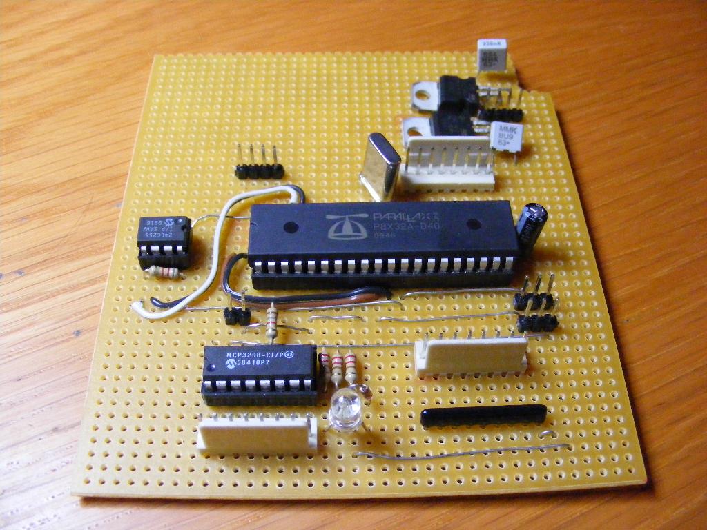
The picture is a little old. Since it was made, I have
mounted a few more EEPROM:s to contain more software,
though I don't use that right now. There are also some
more connections to the card.
Here, the board is put in its box, and connected to the
RJ45 connectors:
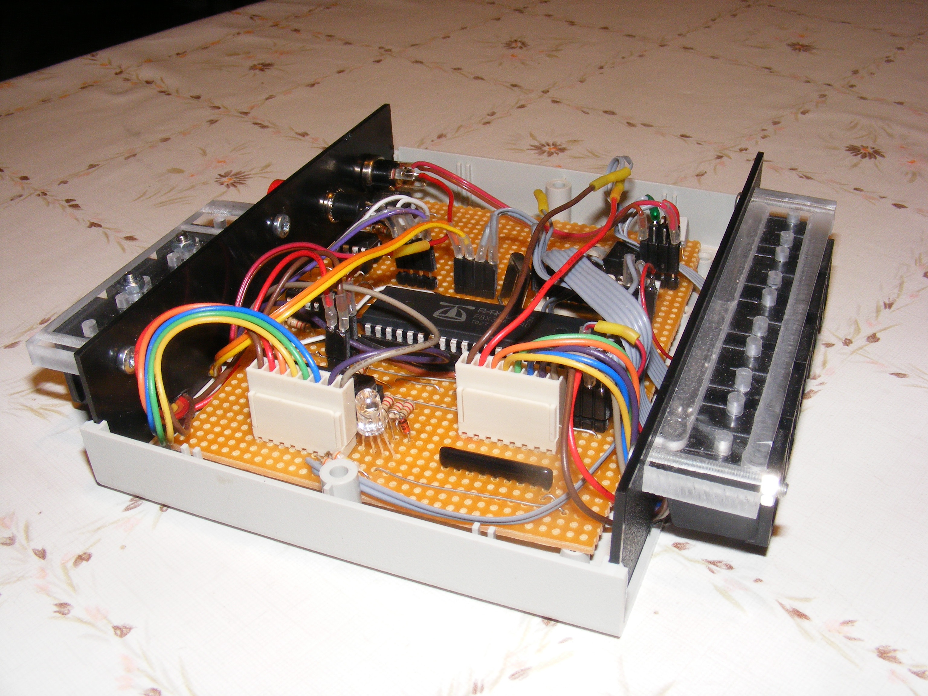
Here is the "programming side" of the box: There is a
power supply input, and a reset button, and then three
RJ 45 connectors. The leftmost of them is for programming
through the FTDI USB circuit. The middle is for connecting
to a similar box containing the RAM memory. The last
connector is for 6 of the analog inputs. On top of the box,
you can maybe see a grey little spot. That is the upper
end of a nylon screw, threaded in the lid, that acts as
ray guide for the light from the RGB LED.
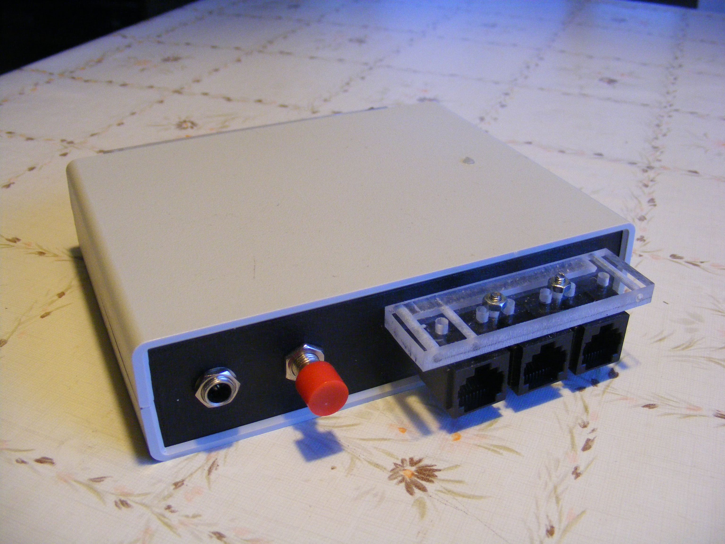
On the other side of the box, there is just a row of
5 RJ45 connectors. The two leftmost are universal outputs
giving acess to 6 Propeller pins each. The second of them
also connect to two analog inputs, for use with the
touch screen. The remaining connectors use fewer of the
outputs. The rightmost connector is for connecting the
keyboard.
Bluetooth has been replaced with Zigbee, but the Zigbee
modem is now outside the box, and connected through one of the
RJ45 connectors when needed. The power amplifiers are
separate units also connected through RJ45.
The FTDI programming unit ("Prop-stick") is built into its
own little box with a USB connector and an RJ45 connector.
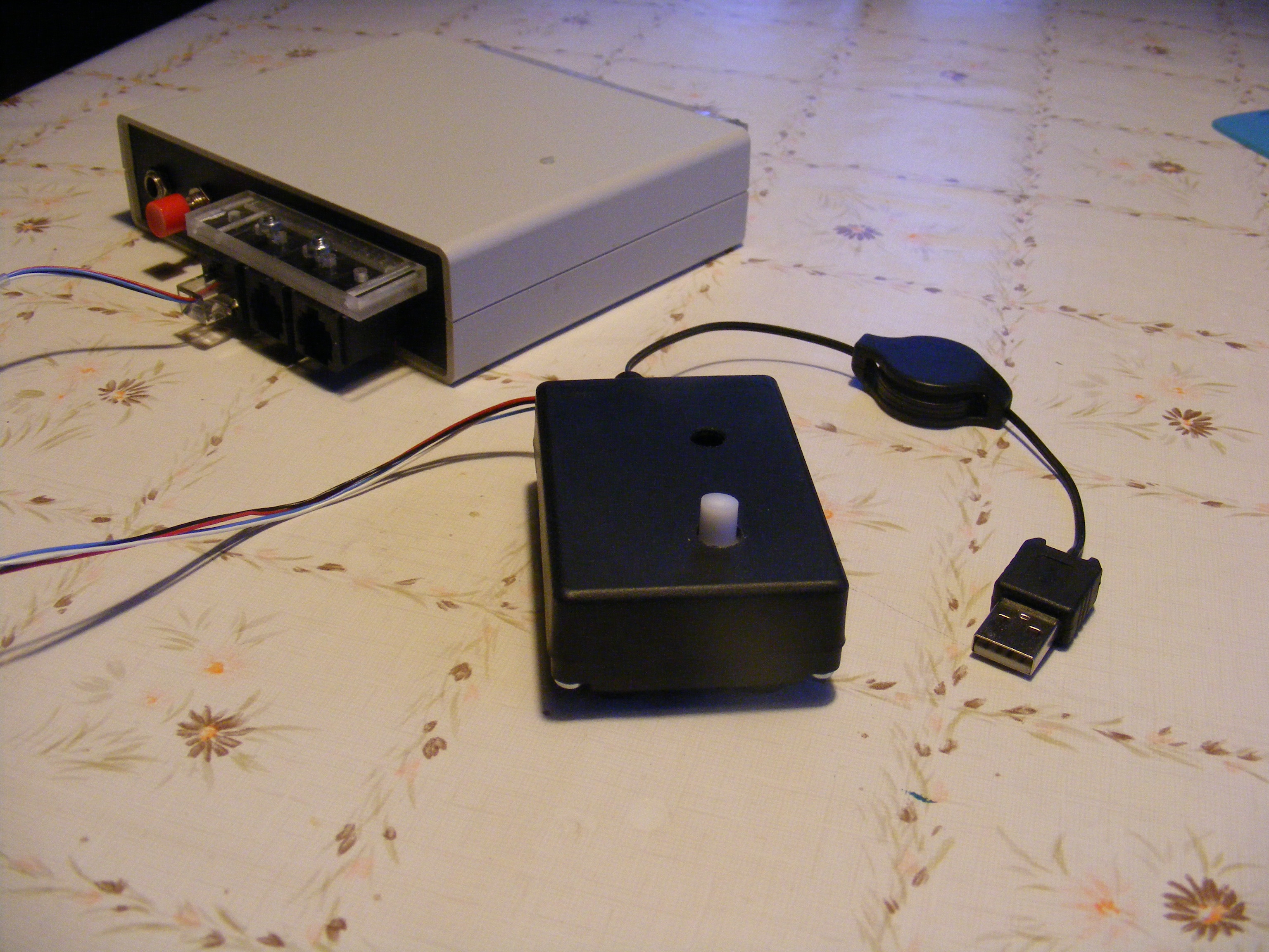
The white button has to be pushed while programming to
enable reset of the Propeller. When it is released, the
box can be used for RS232 communication between the
Propeller and the PC.
The Robot
Everybody who has a Propeller, or any other microprocessor,
wants to make his own robot. Here is mine:
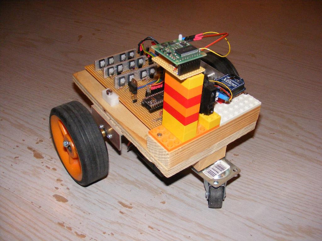
It has two relatively strong 12 volt motors with gear
boxes (1:21), two strong rubber wheels and a caster wheel
in front, and a led battery, that I charge with a CTEK
led battery charger.
It has three power amplifiers. They
are built with discrete components, but they don't work
at very high PWM frequencies, as they get hot. It's OK
for this application to work with low frequencies, but I
don't recommend these amplifiers. The alternatives mentioned
previously are better. Anyway, you can see the coolers for
the transistors as three aluminum bars on the circuit
board.
The computer is a Spin Stamp, which is a surface mounted
Propeller mounted on a hybrid circuit, which also contains
a crystal (10MHz unfortunately, perhaps), voltage stabilizers,
and an EEPROM. On the card, there is also a 3208 A/D converter,
and two voltage stabilizers. One of them reduces the 12 volt
battery power, not to exhaust the stabilizers on the
Spin Stamp. The other provides 3.3 volts for some sensors.
Unfortunately, the Spin Stamp doesn't make its own
3.3v voltage available externally.
In the front, there is a Lego block, on which I can put
sensors and other stuff, mounted on small Lego blocks.
In the picture you can see a compass, mounted on a high
Lego tower, to keep it away from the magnets of the
motors, an infrared distance sensor, and a "proto Zigbee"
unit. The whole robot is controlled over proto
Zigbee from a remote control. I also have an infrared receiver,
adapted to an infrared LED modulated to 38 kHz with a
Propeller computer. So, there is an infrared control for
the robot, but it requires that you direct the LED
pretty accurately towards the receiver.
One thing I don't have is odometry sensors on the
wheels. I once had that. You can read more about
that in the description of the
milling machine.
I am a specialist in autonomous control of unmanned
vehicles, but as this is a hobby, I have made a robot
completely free from all autonomy. It is a remotely controlled
vehicle, basta! But I did some experiments with a
software, that would drive the robot to the nearest object.
But that is not ready yet.
Otherwise the robot is pretty robust, fast and strong,
though it can't compete with modern radio controlled model
cars with brushless motors.
Here's the software
RobotZ.myr
The first thing you notice is a "10 MHz" tag. That's
because the Spin Stamp has a 10 MHz crystal, while the
standard is rather 5 MHz. The Spin code, that is generated
from the MPS code has to know that. So the MPS code
uses the "10MHz" tag to modify the Spin code.
The process input receives the input from the Zigbee
unit. It's a single number comm whose bits
signal which buttons on the remote control are pressed.
The process motor's main program decodes comm
and sets two motor masks and a velocity. The motor masks
are each of two bits, and determine whether the motor
will run forward (01), backward (10) or be stopped (00).
The velocity is set lower if we turn the robot left
or right, and higher when we drive forward and backward.
This facilitates the driving. In the main program, there
is also a call to a heading control function, heading,
which drives the robot to
a given heading, as measured by the compass.
The motor is finally controlled by the function
drive. It sets the PWM duty cycle according to
v (16 is full speed, 100% duty cycle). The motor masks
merged together with shifts and an or instruction are
sent to the amplifiers during the on period, and 0 is
sent during the off period. The total cycle time of
the PWM signal is 80000000/100 ticks, which gives a
repetition frequency of 100 Hz.Fortunately we don't
hear any 100 Hz tone from the motors, probably
because of the inertia of the wheels.
The compass process catches the signal from the
compass, which amounts to measuring the length of a
pulse, that the compass electronics sends regularly.
The scaling i 100μs/degree.
Finally a word about the heading control function
heading. The control error is basically
psi - psiC where psiC lies on
the stack, and the measured heading is a global
variable. But just subtracting angles is a little
dangerous. 1 degree and 359 degrees are only 2 degrees
away from each other, but the subtraction would
give 358 degrees. So we have to "normalize" the result to
within ±180 degrees, by adding or subracting an
appropriate multiple of 360 degrees. Then we control
the motor mask with the sign of the control error,
and we control the velocity with a ramp function of
the absolute error. (We use the || assembler function).
The ramp function is difficult to trim, due to the
friction of the motors. The motors don't run at all
if the signal to them is too low. That is also why
I haven't succeded yet with my "drive to the nearest
object function".
The remote control
The remote control is a box with buttons, a Propeller
computer with its crystal and EEPROM and a proto Zigbee
unit. It is driven with a 9 volt battery. At the back
side there is an on/off switch and a programming connector.
(This figure is slightly old, so it still has D-sub
connectors rather than RJ45 connectors)
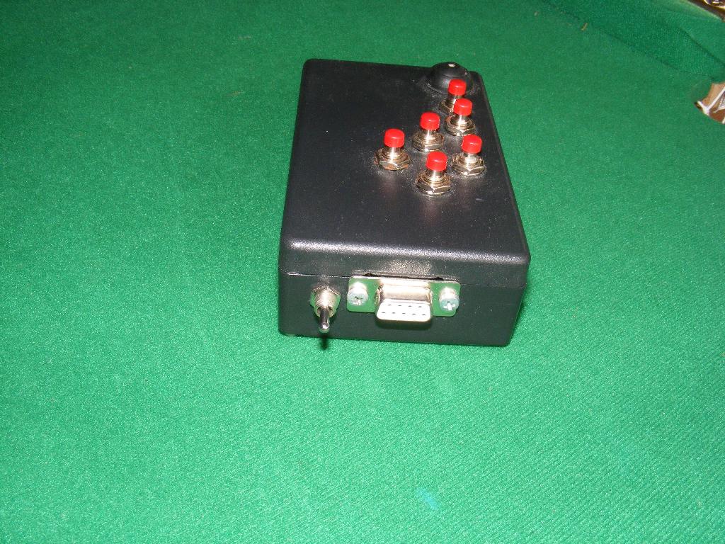
There are 7 buttons, which is less than 8, so the whole
button pattern can be sent in one byte. For that, each
button is connected to its own Propeller input pin.
Download remote.mps.
Download zig.mpo.
The Wheel Steamer
This picture shows the wheel steamer
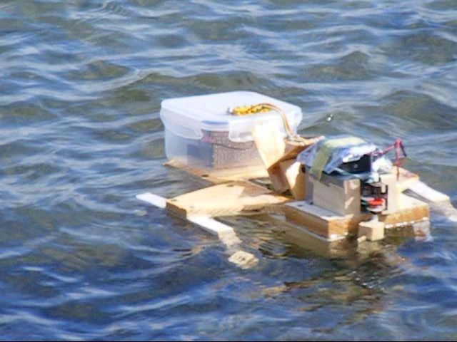
I built it together with my son, when we were in the
countryside
with limited technical resources. You can see, perhaps,
that we are not exactly any expert naval architects.
The ship is built in fur wood, and not plastic foam, so
it is rather heavy. To keep it afloat, it is not a katamaran,
but a pentamaran.
We found a small DC-motor as a main motor. To keep it away
from the water, you can have a propeller with a long shaft,
or a belt drive. But a wheel steamer was also a way to
bring the motor up. We have only one drive wheel, placed
in the middle of the ship, and built around a square hub.
Control is made with a rudder, which is driven with a little
gearbox kit (for those who want to learn what a gear box is).
It gives a slow enough movement to make the rudder
controllable.
We also found a waterproof lunch box, in which we mounted
the electronics, which consists of a proto Zigbee module,
a Spin Stamp module, and a TDA2050 based power driver.
I don't publish any software here, as it is essentially the
same as the software for the robot, although we have one
drive wheel and a rudder here, while the robot has two
drive wheels and a passive caster wheel.
Stepper Motor Robot
A robot equipped with stepper motors has the advantage
that it moves with precision - as long as the hold torques
of the motors are not exceeded by obstacles on ground.
Hence, it is possible to build a navigation system based
solely on the commands given to the robot. The simplest
case is if the robot moves in either of two modes: forward
motion and turning. As long as the robot turns, you just
to update its estimated heading. As it moves forward
you can update its position in the direction of its heading.
But you can generalise this to any type of control. Then
when the robot knows where it is, you can design control
algorithms to go to given points, or to follow given tracks.
Right now, I have just designed the robot, and connected it
to the Zigbee receiver to receive commands.Here it is:
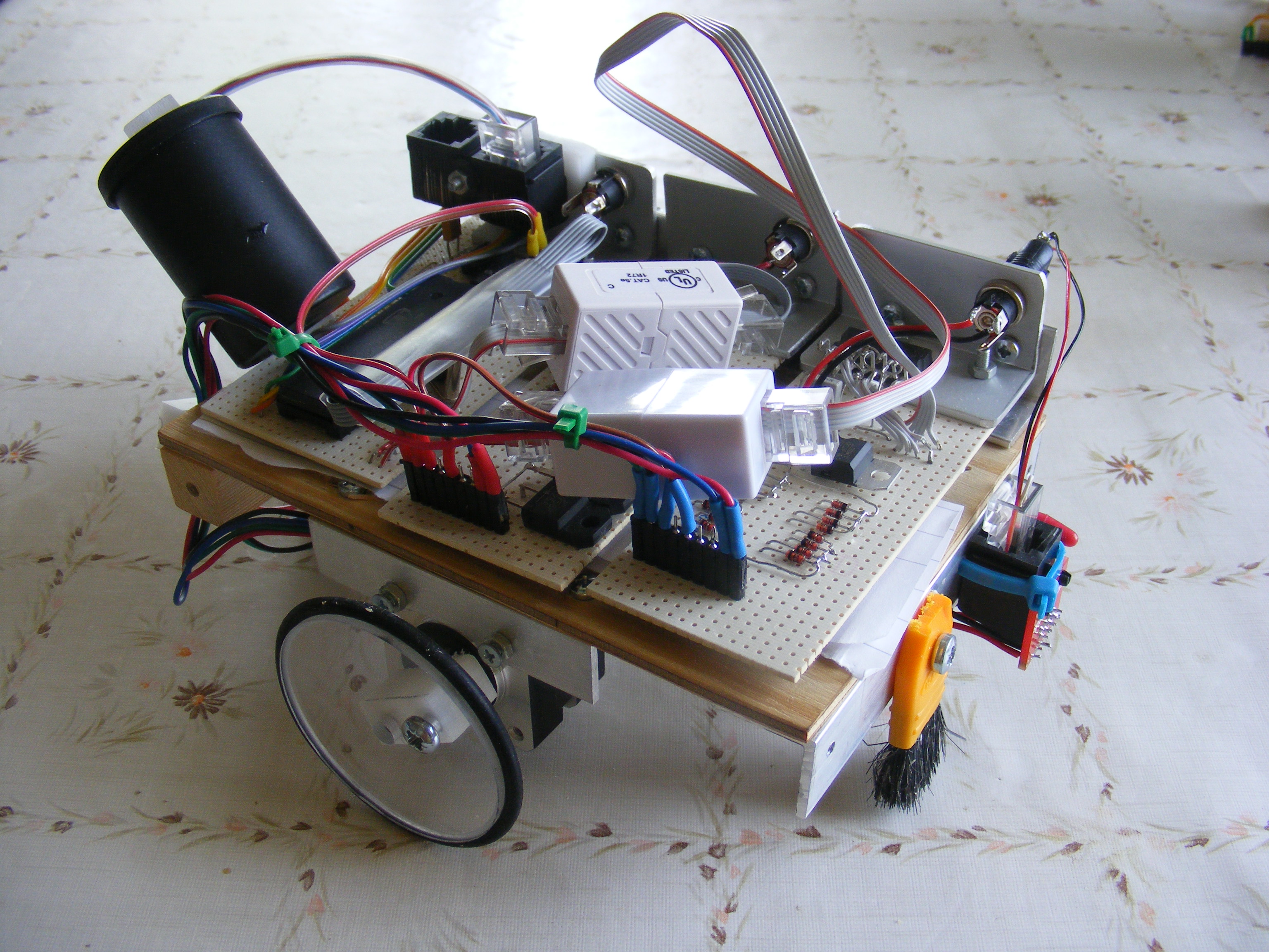
The stepper motors expect a voltage of 7.4 volts and pull
280 mA. For that the hold torque is 650gcm. It is not
terribly much, so the robot behaves best on a plane floor.
The robots are driven by two Lithium batteries connected
in series. They are wired in such a way that they are
charged in parallell which seems to work. Don't try to
charge them in series. If you do that, you need a balancing
cirquit. Also don't charge them with anything but a
Lithium battery charger. Otherwise, you risk overheating
and exploding batteries. The wheels are made in plexiglass
(in fact the other wheel is made in delrin, as I had ran
out of plexiglass), which is cut round and the smoothed
in a turning lathe, and surrounded by O-rings. I use my
standard motor driving cards (you need two for two stepper
motors) and a third card with the Propeller and the Zigbee
receiver mounted in an old Kodak film can. As I use my
standard cards, the wiring looks pretty messy. The robot
balances on two brushes. which makes it an excellent home
cleaning machine.
Here are the programs to download:
stepper.mps.
stepper.mpo.
zig.mpo.
Note how simple the main program is, as it uses the
object file stepper.mpo so effectivly.
The Force Arm
This is a project that requries a good deal of mechanical
skills. Nevertheless it is quite interesting.
A force arm is used in virtual simulators to provide
mechanical feedback to a user, who otherwise gets his
feedback from looking at the computer screen. If the simulator
is for education, the force feedback can enhance the learning
a lot. The situation is that the operator holds some sort of
"pen" in his hand. On the screen he can see in a perspective
image the tip of the pen together with different
obstacles. When the tip touches an obstacle, a force should
be fed back to the operator through the arm.
Such an arm is not an easy thing to make, and the ones
on the market are quite expensive.
The normal principles of force arms, is to provide
forces from torques of motors. Big forces require big
torques, and that requires big currents, even though the
motors have a special design to provide high torque. The
high current problem also induces a cooling problem. If
you try to use a gear box to provide more torque, you get
a new problem: friction. You would drive the gearbox
backwards, to speed up the motor, and that gives a lot
of friction.
The story has a connection to the Swedish Gripen aircraft.
Some experts argued strongly that the pilot must be given
a force feedback in the control stick, so that he could
feel what he did. But the cooling problems forced the
decision to leave out the force feedback in the stick.
I don't think that was terribly important, but after an
accident, some people claimed that the lack of force
feedback was a major cause of the accident. I think they
were wrong.
My idea is to use geared DC-motors! I think you can come
around the problem of friction, by measuring the torque,
and creating a feedback from that to the motors. The
result is an arm, that is worse than professional arms,
but after some work, it is still quite good, and I think
it may be useful for many things,
If you have a force arm, you also have a robot arm, which
can move around to different positions automatically, and
you can do this with different methods, and also combine
position motion and force control.
Here it is:
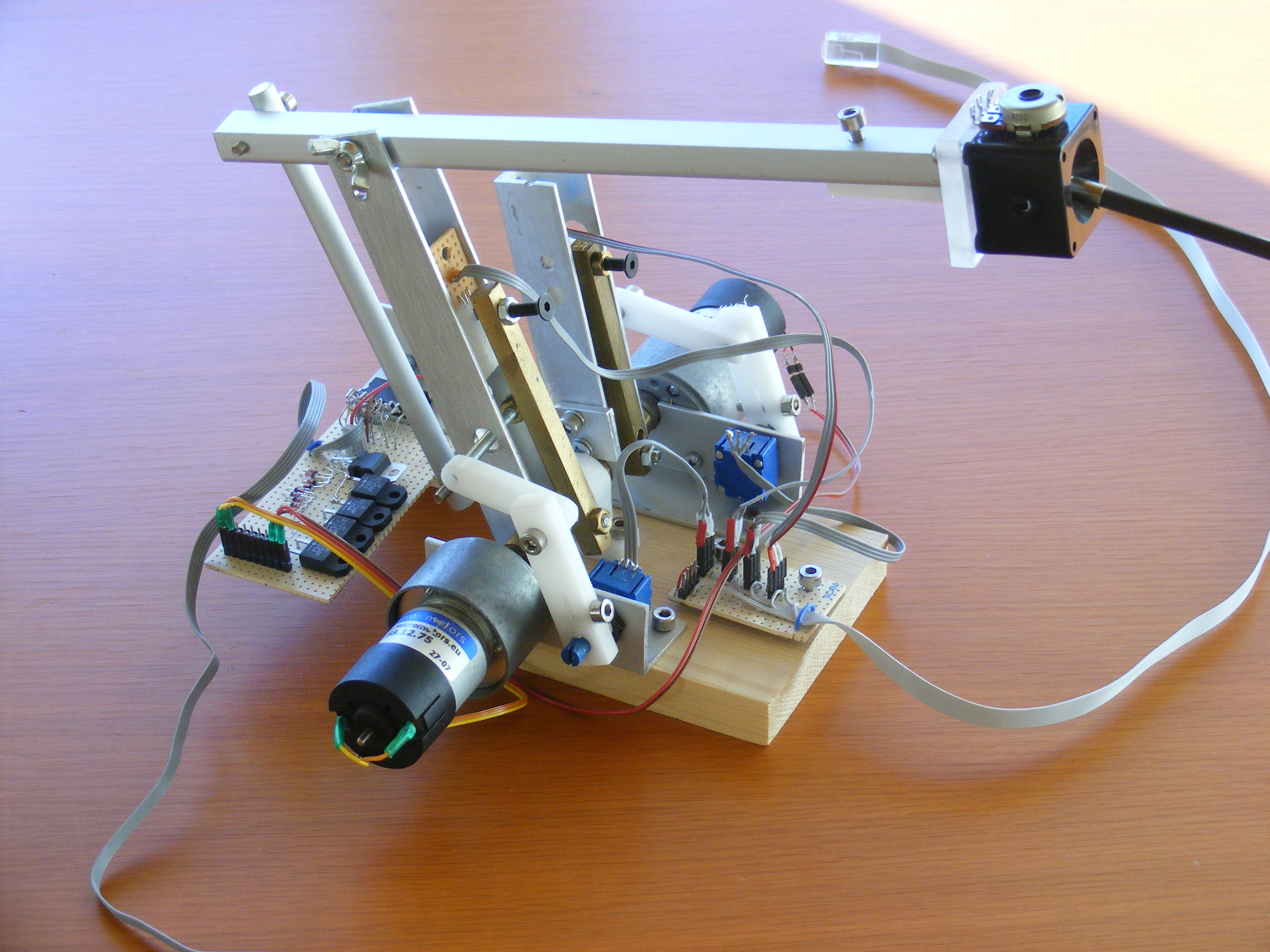
Maybe you can see that it is only a two dimensional arm.
Everything moves in a plane. The way to create 3 dimensions
is probably to mount the whole arm arrangement on a plate,
and move that around a vertical axis.
You can also see the stick or "pen" sticking out from the
arm. It is connected to a joystick, so it would be possible
to measure the angles of the pen relative to the arm,
but I haven't done that yet.
So our first task, is to measure torque. What is torque
(moment in most other languages)? Well, if you mount a
lever arm on a motor axis, you will note that the length
of the arm is important. If you have a longer arm, you get
smaller forces. So any motor is characterized by the
product of the length of the lever arm, and the force
generated at the tip of the arm.
This product of arm length and force,
is called torque. If you have a fix lever arm length,
measuring force is the same thing as measuring torque.
There is only a fix scaling between them.
I argue strongly, that the only way to measure force, is
to give after for it. You let the force act on a spring,
and then the spring is deflected, and you can measure
the force by measuring the displacement. Ideally, you can
have a very stiff spring. That allows you to measure forces
with very little displacement, which may be a point. But
then you must be able to measure very small displacements.
So, probably there is a balance to reach. In my arm I use
a flat spring, consisting of plexiglass! It may seem to be
a pretty odd material to build springs of, but I think it
works. So, the torque bends the plexiglass spring, and
you want to measure how much, by measuring a displacement
caused by the bending. How do you do that?
Not long ago, I tried a so called pressure sensor, which
is a thin film device, which changes its resistance
depending on pressure. In that case, the displacement is
very small. But I found that they weren't very stable.
For the same constant pressure, their output varied
pretty much over time. Further, they don't measure negative
pressure, so you have to make some mechanical arrangement
to bias them with a constant pressure.
Another idea I had, was to use an optical reflex detector.
It has an LED as a light source, and picks up the reflected
light with a photo transistor. If you have a white surface,
they should give a high signal. But not if you place the
sensor too close to the surface. Then efficiency goes down,
and you can measure the deviation from the ideal distance.
It works fine, but the noise level is pretty high.
The next idea is to use a magnetic field sensor, and a
magnet. When the magnet comes closer to the sensor, the sensor
gives a stronger signal. It is a very non linear relationship,
but you can find a range, where the relation is linear
enough. The sensor is based on the Hall effect. The whole
sensor is a little integrated circuit. You need to
find a linear circuit. Most circuits are logical circuits,
which can only distinguish between magnet and no magnet.
The magnet can be a neodynium magnet if you want something
small, and as long as you can afford one; it is said that
the price for neodynium is going up. The signal has a
reasonably low noise level, and as long as you manage to
build a stable mechanical system, they are stable over
time. It is important to mount the sensor firmly. If you
put it on a small circuit board, and let it hang in the
wires, you will get stabiltiy problems.
Here's a primitive drawing of the arrangement:
Distinguish between the arm and the bar!
The arm is a U-shaped aluminum profile. It hangs over the
axis, which is a brass cylinder. The axis has
a diameter of 12 mm, so this is the size of the holes
in the arm, but they should be made with some precision,
to avoid backlash. The motor's
axis enters the axis through a hole, and is locked
to it with a stop screw.
The axis is flattened on two sides.
To it, the plexiglass spring and the bar are fixed
with a common through-going screw. Note, in the left figure,
how there is a u-shaped hole in the arm to give place
for the screw. The other end of the plexiglass spring
is attached to the arm, but with a washer or two to
avoid that the spring lies flat on to the arm's surface.
The bar is a square brass rod. This is nice and
stable. Aluminum might work, but maybe not plexiglass.
At the end of the bar, there is a steel screw, which the
magnet likes to adhere to. The magnet can be moved to
an optimal position with the screw, and then the screw
can be locked with a nut. The bar moves relative to the
arm, as the spring is bent. This is measured by the sensor.
The sensor I found is a trapetz shaped little thing. I've
mounted it firmly in a hole in a piece of plastic, which
is screwed to the arm. The hole should be
close to the surface, so it may be easiest to make the
hole first, and grind away material afterwards.
The sensor has three pins. Solder a ribbon cable to them
and lead that down the arm to the electronics.
This is one arm unit. To get a double arm, to allow
movement in the plane, we could put the next arm at
the tip of the first. But the weight of the arrangement
would probably be forbidding. So we mount the second
unit at the same base plane, and then connect that
unit to the second part of the arm through a mechanical
link. This is easy, if we mount the two units so that
they have common axis line, i.e. the two motors are
coaxial.
The link arm is a round aluminum rod. It is tied to
an aluminum plate, which goes out from arm #2 in a
right angle. For these links I use screws, that are
tightened to one of the members, and threaded into the
other. You can see this arrangement here:
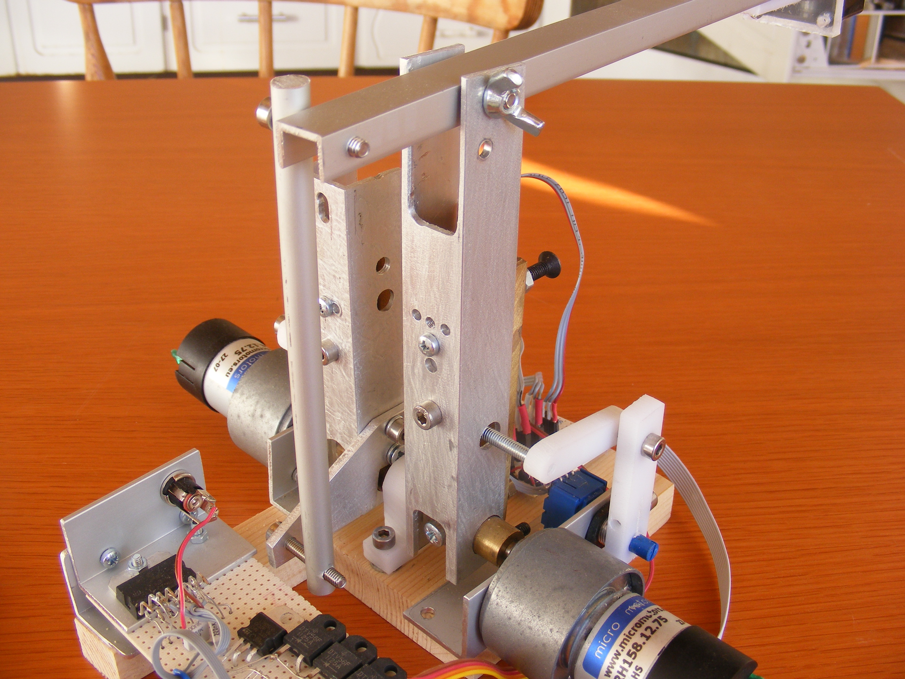
The motors axes are somewhat unsteady, so I have built
a little support block in plastic where the two brass
axes can rest. You can see this in this pictures:
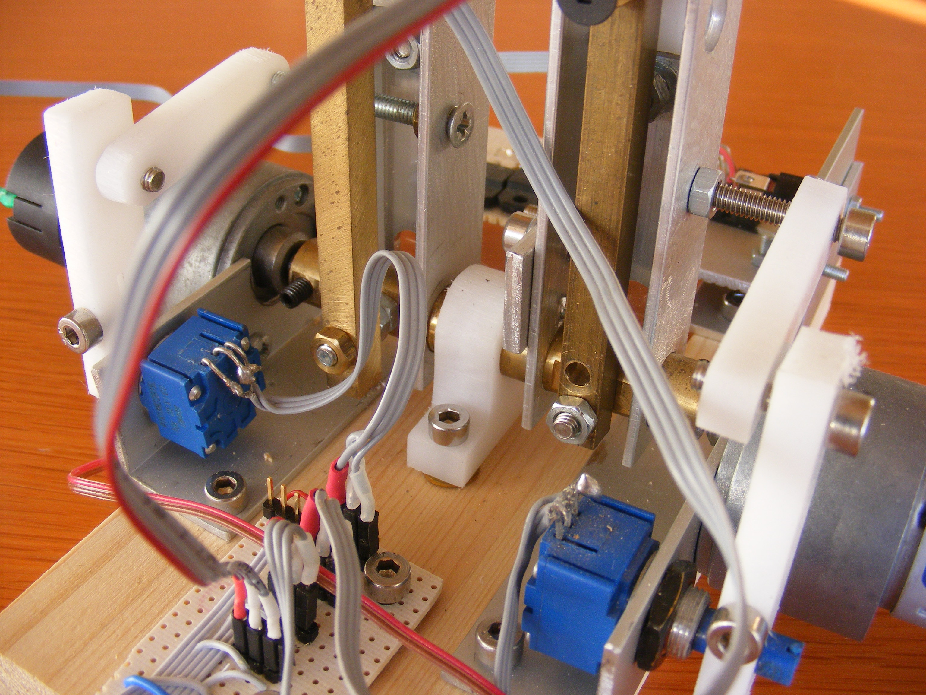
Schematically, we have this arrangement:
The little circle marks the end of the arm at position
(x,y). From there, the arm acts outwards with a force F
with the two components (Fx, Fy).
The position of the arm is controlled by the two angles
α and β. Note that with the link arrangement we have,
the second arm unit controls β directly. If we had put
the second arm unit at the tip of the first, that unit
would control β-α, which would be more difficult.
Now we realize, that we need to measure α and β, which
we do with potentiometers (if not anything more advanced).
But as the motor are coaxial, there is hardly space
for any potentiometers directly coupled to the motors,
so we have a link arrangement to drive the potentiometers.
Look at the photographs to see these link arms in white
plastic.
A somewhat open issue is whether the potentiometer should
be connected to the motors or to the arms themselves.
The good side of connecting the potentiometers to the
motors, is that we entirely eliminate the friction of
the potentiometers. But there is a slight difference
in position between the motor and the arm. When we
build feedback loops around the arm, this difference
can easily destroy stability. Here we have connected
the potentiometers to the arm, and hence we should look
for potentiometers with low friction.
Now, some mathematics. We can compute x and y as:
x = l1cos(α) + l2cos(β)
y = l1sin(α) + l2sin(β)
So this is a function that we would implement in our
system, so that we could base the computation of forces
on position.
But you could also differentiate this equation, to get
the relation between the rotational rates of the
motors, and the velocities of the arm tip. But it
is even more interesting to invert this relationship.
The differentiated equation is linear, and so it is
described by a matrix. That matrix can be inverted. In
doing so, you need the determinant of the matrix. It
is (after using one of these trigonometric rules):
D = -l1⋅l2sin(β-α)
When this is zero, you can't do the inversion. When is that?.
Well, it is when α=β. In that case, the arm is fully
streched out. You can wave with the arm, but if you
want to move the tip of the arm closer, it takes a great
change in α and β. Here, then is the equation:
ω1 = (1/D)(vxl2cosβ+
vzl2sinβ)
ω2 = (1/D)(-vxl1cosα-
vzl2sinα)
So now, given a velocity (vx,vz)
that we would like to give the arm tip, the equation
gives us the rotations we need from the motors. Typically
we control these just by the voltage supplied to the motors.
We may think that we have a goal point of the arm tip.
We can compute (vx,vz) so that it is
directed straight from the current position of the arm tip
to the goal point. We have to scale the velocity, so that
it depends on the distance. Now, when we start the
feedback, the arm would ideally move from any point to
the goal point along a straight line. It doesn't quite,
because of the transient behaviour, when the motors speed
up. Also saturations in the motor control amplifiers will
alter the behaviour. But sometimes it works quite nicely.
This is called kinematic control.
Before we go to dynamic control, we should mention shortly
geometric control. Then, given a position that
we would like to move to, we can use our first equation
to compute corresponding angles α and β. It is a
computation, that involves arctangents which is a little
complicated, but it can be done. Then we construct a
feedback from the α and β potentiometers to the motors,
to bring α and β to the desired values. The motion of the tip
is not along a straight line
and it is hard to compute the exact track over long
distances, but of course it works.
Dynamic control is about controlling forces, and
that is what we started to talk about. So the question is:
What is the relationship between the torques of the motors,
and forces at the arm tip? It doesn't sound all that trivial,
but it is almost trivial, if we think about a situation of
equlibrium. Let's grab the tip of the arm, and hold it
firmly, to prevent any motion. The forces it takes to
hold the arm are exactly the force by which the arm presses
onto my hand. If I released my hand, the arm tip would
move just as if it were affected by the same forces.
The forces from the motors, and the forces from my hand
are the only forces present, except gravity, which is
negligible. So we let my hand be there, and compute
the balance between the hand forces and the motor torques.
Here's the result:
Fxl2sinβ+
Fyl2cosβ = M2
Fxl1sinα+
Fzl1cosα = M1
Here, we don't need any inversion. The equations gives us
exactly what we want. Given some force
(Fx,Fz) that we want at the arm
tip, we can compute the torques immediately, and we can
achieve these torques through our torque feedback
mechanism.
Then we can make a position feedback by computing a
force from the deviation in position. But that't not
necessarily a good idea. But, let's go back to the
original idea, of pointing at a "virtual object" on a
computer screen. When we touch the object, we would
get an outward force. But that is a feedback from position
to a force. And back from the force to the position,
there are two integrations. So, there is no damping.
Fortunately, the inner mechanisms in motor control helps
contribute with some damping. The motor current controls
torque. And the motor current depends on the applied
voltage and the winding resistance. But not while the motor
moves. Then the generator effect of the motor is in
charge, and it reduces the current. This helps up
stability.
But what happens in real life? Well, if you drop a metal
ball on a table, the ball suddenly experiences an
upward force. So it accelerates upwards, and then it
bounces. But the bouncing stops, because some energy
is absorbed in the table and in the ball at each hit.
And this has to do with the characteristics of the
forces that repell the ball away from the table.
With a force arm, we can attain stability, by designing
the repelling forces somewhat smoothly. But it doesn't
work unconditionally. If we hold the arm firmly, we can
usually get a good behaviour, but if we hold the arm
more loosely, it can start oscillating. Manufacturers of
expensive force arms claim, that they have solved this
problem, but I remation sceptical. The problems are
very fundamental consequences of ordinary mechanical laws.
Now to an application: The window cleaning robot.
The normal engineering approach to this would be to have
the robot arm tip move over the plane where the window is.
Then it would have some brush or so. But if the window is
just slighly closer than we thought, we would crash the
window. And if it is just slighly farther, we would just
clean the air. What we want is a given force normal to
the window, to press the brush against the window for a
good result. In the remaining dimensions, we would move
over the surface of the window. So we want dynamic control
in one direction, and we would perhaps prefer kinematic
control in the other two. But as far as I have understood,
it is difficult to mix dynamic and kinematic control. So
we must work with dynamic control throughout. It's OK.
We can control position through force feedback. The
friction of the window will provide us with damping. We
keep imagining that we have a three dimensional arm, so
we have a force vector of
(Fx,Fy(x-xc),Fz(z-zc))
where (xc,zc) is a position that slowly moves over the
surface of the window, while Fx is a constant
force suitable for window cleaning.
As you know, I just have a two dimensional arm, so I can
just clean a one-dimensional window. Furthermore I have
laid the window down, so this is maybe a factory facility
for cleaning windows before delivery.
Here's a picture of the setup:
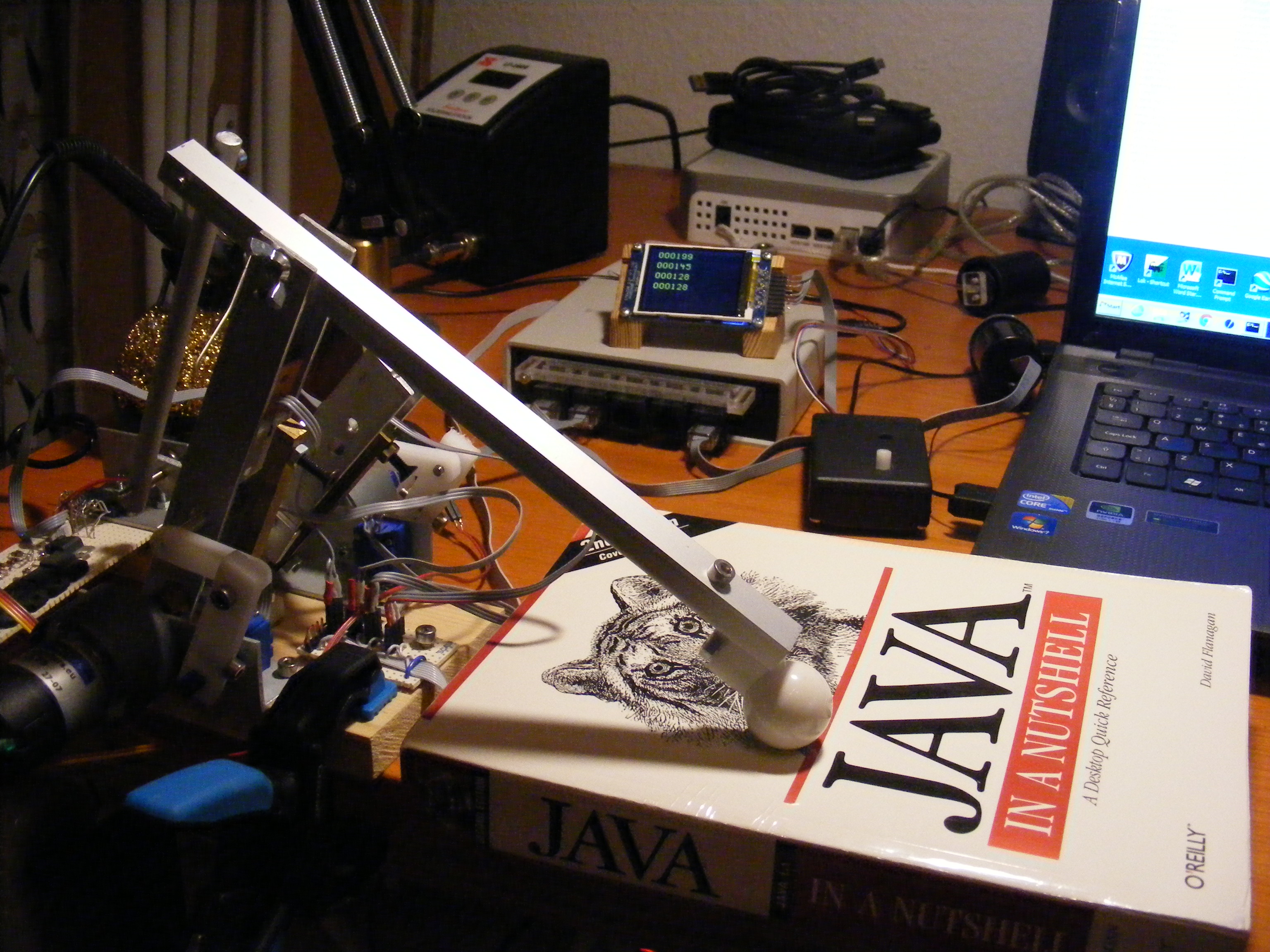
As you can see, the window is not even a window any more,
but a Java book. And the pen and joystick arrangement
has been replaced by a bullet. (There is a workshop
technique for making nice smooth metal sufaces, by
pressing a bullet against the surface. In Swedish, it
is called kulpening, which sounds funny even
in Swedish.)
Here are the downloads:
I use the keyboard to control the arm, and some data are
presented on the display. For the keyboard, '4' turns the
motors off, and they are turned on with '6' and '7'. Before
turning them off, you should use '0' to remove biases from
the torque sensors. While you do that, you should leave the
arm in peace.
The main program, Arm2D.mps, needs a little overview.
With the exec line, as it is written, the arm runs
in dynamic mode, through the process posforce which
means force as a function of position.
Before that, the signals from the torque sensors are
collected in an which also collects the angles
α and β. All this comes from the A/D converter. The
function debias finds the 'null-value' of the
torque sensors by low pass filtering the signals. The
low pass filtering requires a temporary upscaling of the
signals with a factor of 26. The process
pos computes the position of the arm tip, but the
process also computes some goal positions for the arm
tip. There is a circle, and a track between some given
points (a function called bana, which means track).
Posforce then computes a force in terms of two
components fxc and fzc. From them, the process computes
the corresponding commanded torques m1c and m2c. There are
some functions to choose between. Brushforce is for
the window cleaning task. That function also maintains the
position over the "surface" of the window, where the arm
should go, and a force is produced to move it there.
Noforce is good to start with. It produces a zero
force. If everything works, it should be very easy to
to move the arm. Boxforce produces forces to force
the arm tip into a box. This is the major test of the
arm as a force arm. Refforce is the way to move
the arm around the series of points produced by bana.
The torque feedback is made in the process momfb
which compares m1c and m2c with the torque sensor signals
with bias removed, and sends the results to the motor in
form a pulse width signals. 256 here means full signal
to the respective motors (100% on). The pulse width modulation
is handled by the process pwm, which can handle
both motors simultaneously. The process is compact and
fairly cryptical for speed. The total period time
(on and then off) i 4096 tics, which is an integer power
of 2, which helps making the program simpler.
The second alternative exec line is for kinematic control,
which is mainly handled with the process posfb.
One of the tasks is to move the arm through the goal
points of bana. The other task is more challenging.
I have failed with it, but I leave it to anybody to make
a try. Here's what it is about.
The chua circuit
The chua circuit, built by Leon Chua, was the first
successful try to build an electronic circuit, that could
produce chaos. Until then, chaos had only been made in
computers, though in some cases these computers were
analog computers. I tried to mimic what Chua did in
his circuit with my arm. but so far, I haven't made it.
You have an unstable oscillation around a center. So the
tip of the arm moves in a spiral with increasing
amplitude out from the center. On its way out it will
come close to a second center, and when it comes close
enough, it will switch over to spiral about that
center. As it is now close to its center, the amplitude
of the oscillation will be small. But it will grow.
In this way, the spiral will come close to the first
center, and will oscillate around that. And so on.
The information about which center the system shall
spiral, will have to be stored separately, so it is
a (boolean) state variable. The other two state
variables are the position coordinates. So altogether,
there are three state variables. One can prove that
it is impossible to make chaos with fewer state
variables than three.
So, one would like to see the arm move erratically
around the two centers. What failed to me, was that
my motions around the centers were always much more
unstable than I expected. Probably that is because of
the long sampling timed. Those who know about
Runge Kutta's integration method might do something.
Exact linearization
The dynamic control of an arm is actually a special case
of a procedure called exact linearization. There
is an established theory for how this is done and when
it is at all possible by the Italian differential geometer
Alberto Isidori.
Recent developments
Recently, I rebuilt the arm electronics, so that it has
its own dedicated computer. Then I replace the keyboard
with two manual switches, A push button controls the
debiasing of the torque sensors. and microswitch activates
the motors (through software). Furthermore, I have done
away with the display.
I have also built a second arm, which copies the position
of the first (through kinematic control). That second arm
has a little force sensor, whose force signal is fed back
to the first arm. Then you get a force feedback when the
second arm hits something. I'll come back to this at some
later time.
The Milling Machine
I am the happy owner of the milling and drilling machine
you can see here:
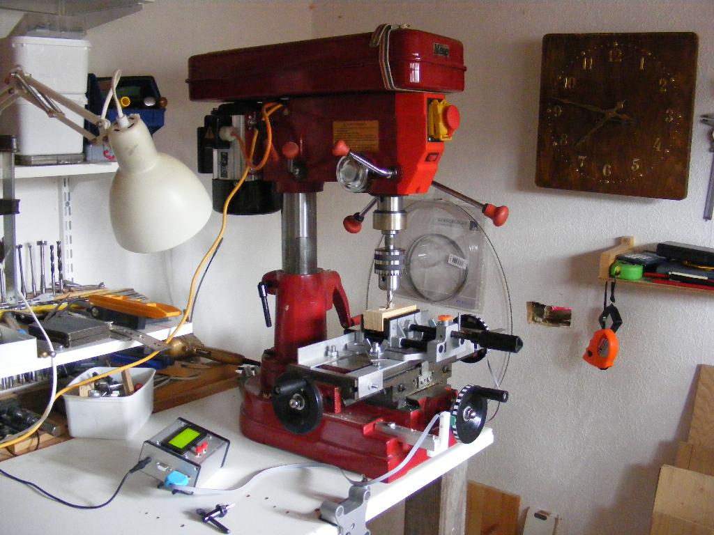
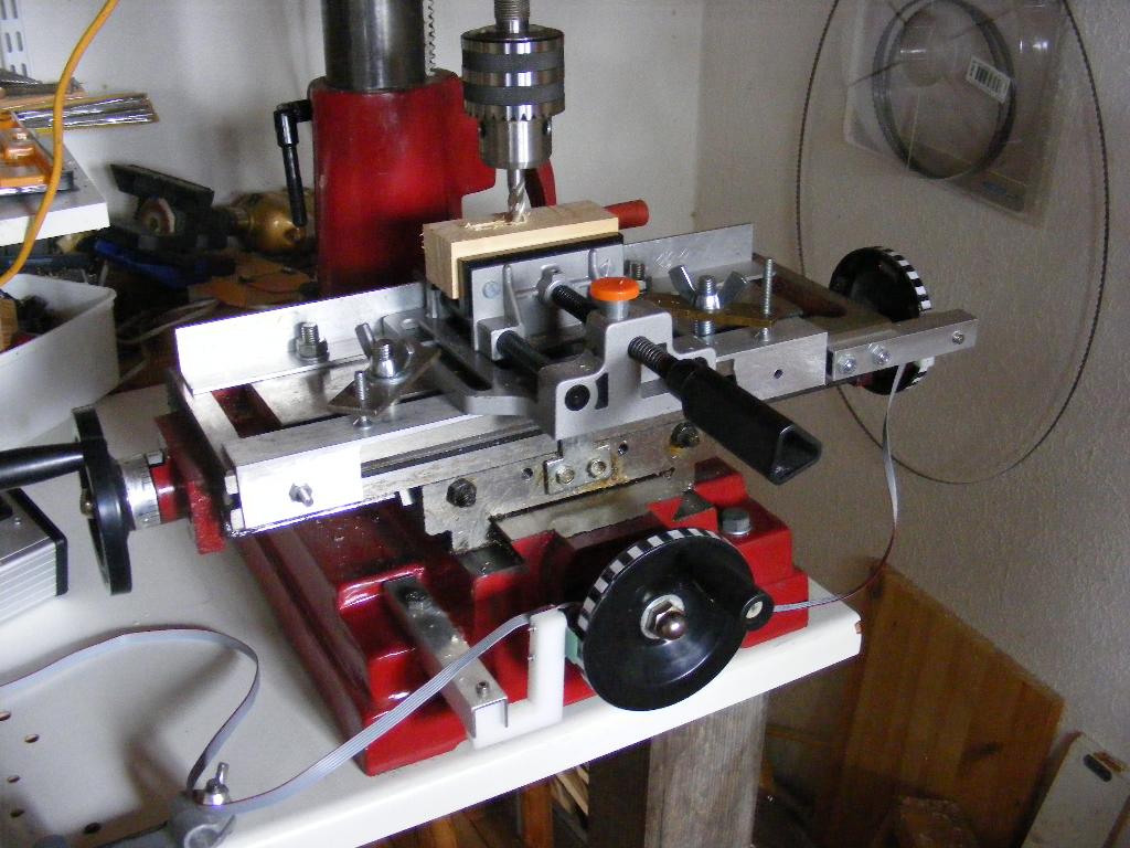
It has a coordinate table with two cranks to move the
workpiece in two orthogonal directions. I have mounted
striped tape on the two cranks, and then I have mounted
a pair of reflex detectors nearby. The reflexdetectors
are from Polulu and intended for odometry. The following
pictures show the arrangement more in detail:
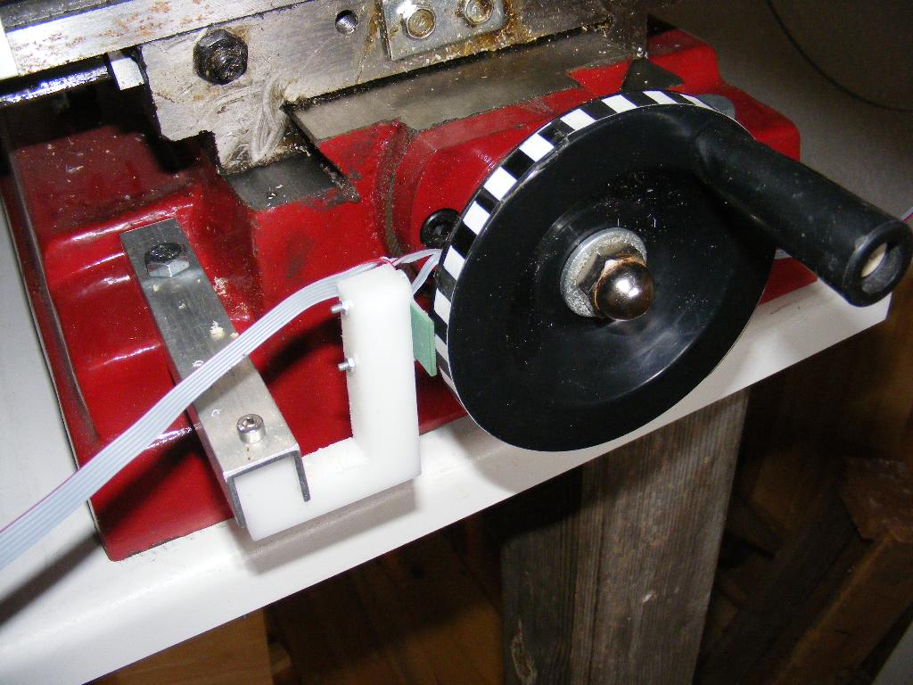
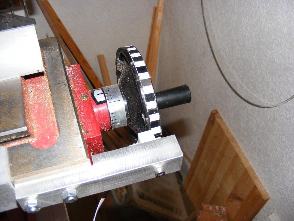
Then i have coupled the reflexdetector to a box containing
a Propeller computer and an alphanumeric display.
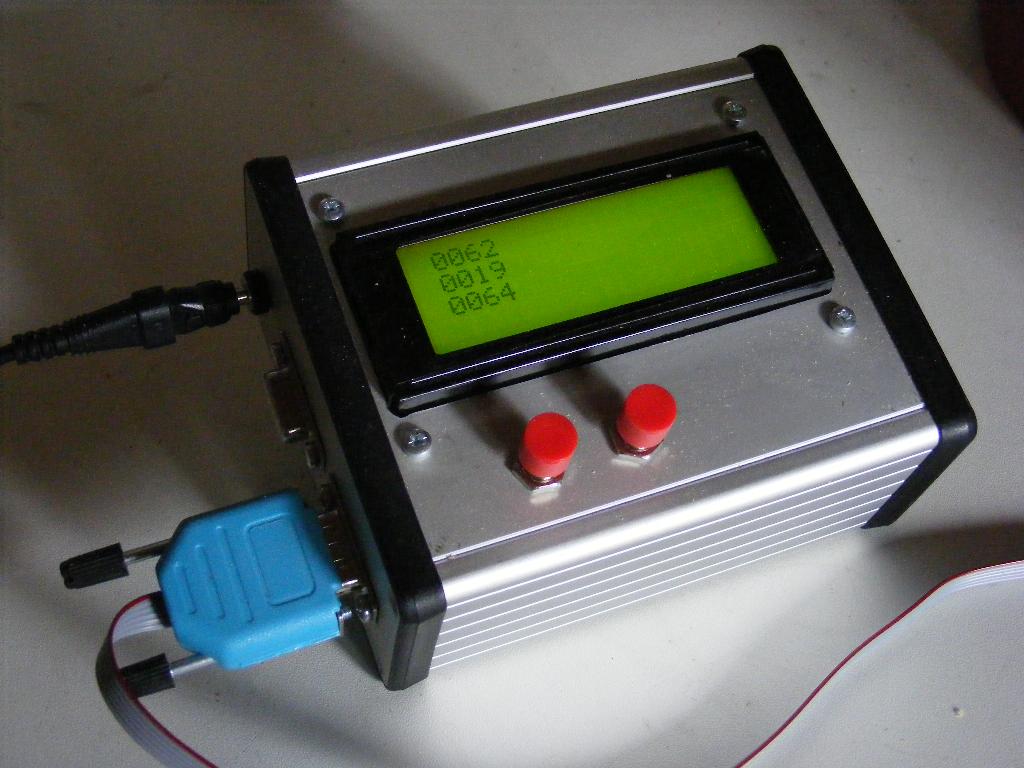
The software consist of odometry computations based on
the odometry object as described above. With the stripes
I have made, the resolution in table movement becomes
1/14 mm, but I have recalculated this, so that I get
resolution of 0.1 mm. On the two first lines of the
display, I show the coordinate table positions in
tenths of milimeter. All coordinates refer to a reference
point, that you set by going there, and then pressing
the right hand red button.
The third line shows the distance to the reference position.
This is computed with Pythagoras' theorem and the
itsqrt function in std.mpo for computing the square root.
This function is of course usefull when you want to mill
out a big circular hole. If the hole should have the radius
R, and your milling tool has the radius r, you should move
out to the distance R-r everywhere, but no longer.
Another thing that you maybe would like to mill, is an
oblique straight line. You could define such a line by
moving to two points on the line, and press the two
red buttons. Then the display could show the distance
to the line. This is a function I haven't made, but it
would be possible.
The equipment is good for milling, but also for drilling where
you could place your holes with good precision. In all,
this is a very nice little equipment, that raises the value
of the machine considerably. Of course, from this point one
can go on and add motors, and make a numerically controlled
machine.
The following picture gives a little instruction for how
to make a hole for a D-sub connector.
Download Odo.mps
Download Odo.mpo
Download std.mpo
Download Display.mpo
The last object file is for an alphanumeric display sold
by Parallax. It lets you type characters on the LCD display
just by sending the ASCII-codes and some command codes.
But, of course, you could also use the Adafruit display
presented earlier.
The USB Oscilloscope
This is a new version of a USB oscilloscope. It's based
on an A/D converter from MAXIM, called MAX118, which is
capable of sampling at more than 1 MHz. It has 8 bits
resolution, which isn't so much, but it simplifies
programming, as the whole result can be delivered in a
single byte. The result is delivered from the converter in
parallel form,
which partly explains the relatively high sampling
frequency.
To use that speed. requires some efficient
programming. This is done in the panalog.mpo
object file, and involves some preparatory works making
masks for adressing the converter rapidly.
Additionally, the device can log 6 bits of data sampled
directly from the input pins of the Propeller.
Data are then logged in the Propeller global RAM. There
is space for 7000 longwords, which means 28000 bytes.
This is pretty much, so you have good opportunities to follow
what happens in your system under investigation.
Data are sent over the USB to the PC
at the end of logging, and then they can be displayed
immediately with a plot program.
Here's a scetch of the cicuitry:
Note that the inputs to the A/D-converter are not drawn
in the order, they appear on the chip. You have
to consult a data sheet.
To the left, there are 4 different
analog circuits with different properties.
- This input accepts an AC signal through a capacitor.
It has a gain of 10 and an input impedance of 10 kΩ.
The range is moved up from zero to the range of the
A/D converter. Hence the input range is +/-0.25 volts.
- This input has the range +/-2.5volts. So the gain
is one. The impedance is 10kohms.Not super much,
but good for most purposes.
- This input also has the range of +/-2.5 volts.
but it drives current out to the source, which isn't
always acceptable, specially not if you have a series
capacitor in the source.
- This input has the same range as the A/D converter
itself, i.e. 0 to 5 volts. You might think that this input
has a high impedance. but it isn't quite true. The way
the sample and hold circuits in the converter work, your
source can't have a high impedance. But a couple of
kiloohms is OK.
The amplifiers in the circuits are not operational
amplifiers. They are far two slow. Instead I have used
videoamplifiers from a circuit called AD8013 from
Analog Devices. To my surprise, it was possible to
give them a strong feedback without stability problems.
The converter is driven with 5 volts. Its reference inputs
are supplied with 0 and 5 volts, which gives the conversion
range of 0 to 5 volts. But the reference inputs need to
be well stabilized.
The A/D converter is controlled with the CS and RD pins.
When they are set to zero, conversion begins, and when
it is ready, this will be visible in the INT-signal. During
conversion, the adress bits have to be set, so that the
right input signal is converted. The converter is a 5 volts
device, and the Propeller is a 3.3volt device, so the
outputs of the converter have to be delivered through
protection resistors.
There are also digital inputs directly connected to the
Propeller. As they are not protected, you should be
carefull.
But, on the other hand, you could consider to build this
device with
just the digital inputs, and skip all the analog circuits.
A digital data logger is a usefull thing.
The Propeller has a 3.3 volt stabilizer (not shown in the
diagram), crystal and EEPROM connected the
usual way, and the Propstick. That's where we take
out data to the PC.
The program that catches the data builds on the same principles as
Propp.java, which is presented
here, but it is more specialized,
and takes care of the data from the Propeller automatically.
It's called OscNy.java.
When you start the program, you get a square window, from
which you can control the oscilloscope. You do so by
having the window in focus, and typing characters into
it. These command characters are as follows:
- I sets digital mode.
- N sets analog mode
- V sets variable mode (described in the next
section)
- S sets single mode
- D sets dual mode (two channels A and B).
- Ax, where x is a number that selects the input
to channel A
- Bx sets the input to channel B, which
is displayed in dual mode.
- Tx where x is a number between 0 and 5 that
sets the sampling interval to some predefined values.
The result of these choices is displayed in the
window. When you then hit the spacebar, the
program will put together a two byte command, which
is sent over to the Propeller. When the Propeller
gets these two bytes, it starts logging the data in
its global RAM memory, and when the logging is complete
it will immediately send the data over to the PC.
The PC program OscNy.java will capture the data
in a byte array, and then process the data
depending on mode. The data will be brought to a file,
and then a plot program window will appear, where you
can look at the data.
Here's a little how you command this plot. It's mostly
done with the keyboard. In the upper right corner of
the plot window, there is numbered list of the variables
including time. You choose a variable by typing its
number and then Enter. If You type two numbers before
Enter, you will get the the one variable as a function of
the other. While you look at one variable, you can type
the number of another, followed by a p and
followed by Enter. Then you see both variables in the
same plot with a common scaling. Then you can go on
in the same way with a third variable. When you plot
digital variables, the variables will be somewhat separated
vertically,
so that you can distinguish them.
In the lower right corner, there is a little menu of
words, of which one is marked by being red. You can
move in that "menu" with the arrow key, while holding
the control key down. Then you can change the scalings
with the arrow keys. Try this out, to see how it works.
The plot has a time scale, which should be accurate,
because it's based on actual time measurements in
the Propeller before and after logging.
Here are the files for the Propeller program:
Here are some Java files:
But that's not the whole story, for the main program
OscNy.java uses USB, which requires some C programs too.
Refer here for more information
about that.
Plotting from programs
Here's a process and an mpo file for make the same
thing for variables inside your own Propeller software.
This allows you to plot your own variables. Put
the process into your mps program, and mention it in
your exec field. Then you should declare 4 global
variables u0, u1, u2, u3. Then you can write values
into these variables anywhere in your code, and then
these values can be plotted. To do this, open
OscNy.java on you PC. Hit the V-key on your
keyboard. The control window will display the word
"Variable", which means that you display Propeller
variables. In this mode you can't set anything else.
The sampling time has to be set "hard wired" in you
Propeller logging process. Now, hit the spacebar,
and you will see your variables plotted.
The values are stored and processed as bytes. These
are the least significant bytes of u0 ... u3.
In your Propeller program you should also declare
the area where you logg your data as
area[5000]
This area is slightly smaller than the one in Panalog.mps.
The reason is that the program you connect it to may
take up more space in global RAM, and in that case there
is less space for area. In the process itself
there is a variable called size. It should now
exceed the declared size of the array area.
Lately, I've made a new Java program for displaying
variables, sent over USB, visible as figures on the screen.
It also creates a file, that you can plot afterwards.
It is controlled by a control file, that gives variable
names, and information of how the different variables
are packed into the bytes. I will come back to this at
a later time.
The Telescope
When you look at a star with a telescope, the telescope
will rotate with the rotation of the earth. So to get a
stable picture, you have to rotate the telescope backwards,
relative to the earth. Amateur telescopes usually have
something called an equatorial gimbal system, which is
a mechanical arrangement, such that one of the degrees
of freedom falls along the rotation axis of the earth.
There is a knob there, and by rotating that slowly, you
can counteract the rotation of the earth. Equatorial
gimbal systems are a bit clumsy, though. They require a
big counterweight, which makes the whole telescope heavy,
and the telescope tube sometimes makes a pretty awkward
journey, when you direct it against different parts of
the sky.
So the whole project here is about making a virtual
equatorial gimbal system. The starting point then,
is what I would call a "fork gimbal system". The telescope
tube is hung up between the arms of a fork, and can
be moved up and down there. This is called the elevation
movement. Then the fork can be rotated around a vertical
axis. This is called the azimuth movement. The problem
now is to distribute the counterrotation against the rotation
of the earth to the two axes, azimuth and elevation.
Here is a picture of the fork gimbal arrangement:
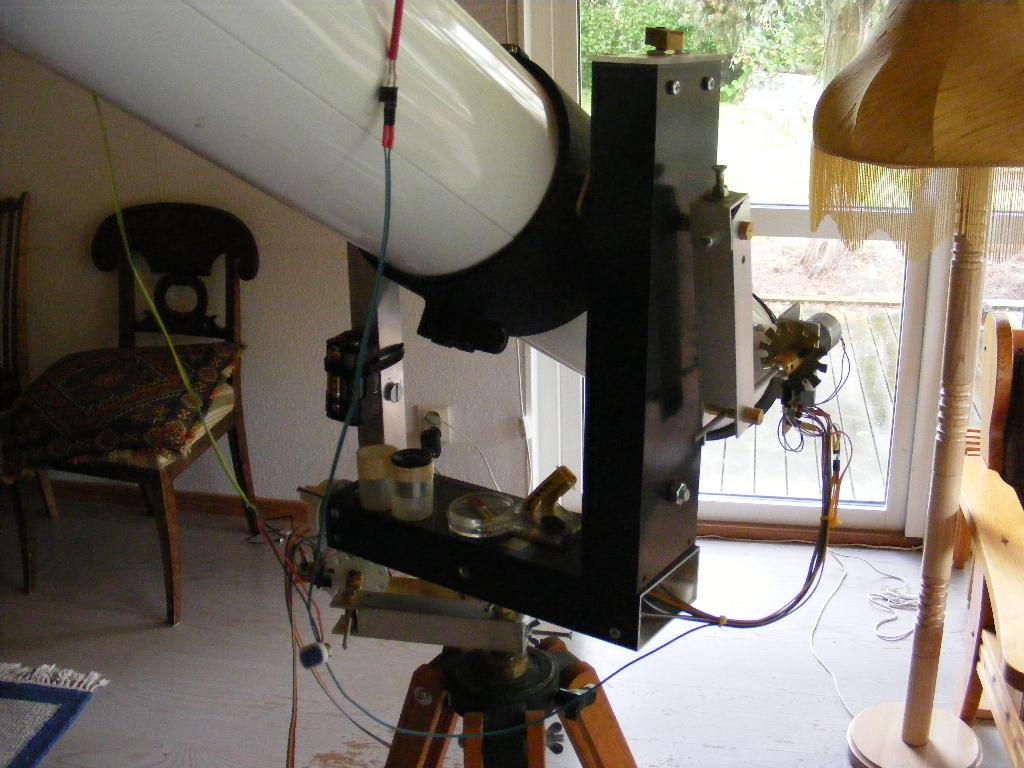
First of all, the rotation of the earth is directed towards
north, and it is tilted up from the horisontal plane with
the latitude of the place. So on the equator, the rotation
axis is lying down, and at the North Pole it stands right up,
so the direction towards north doesn't matter, which is lucky,
because there is no notion of north at the North Pole. Then,
there is a more tricky mathematical problem. The azimuth angle
and the elevation angle are so called Euler angles. There is
a third Euler angle around the axis of the tube. So what we
want to control is time derivatives of the Euler angles,
and what we have is the earth rotation vector. But the
relation between rotation vectors and Euler angle derivatives is
a little bit involved, and it is easy to make mistakes there.
But I provide you with a Java program that solves the problem.
The result shall be a function with three inputs:
- The latitude of the place.
- The elevation angle
- The azimuth angle, measured relative to north
... and two outputs
- The time derivative of the elevation angle
- The time derivative of the azimuth angle
The motions involved are very small. The earth rotates
1 full revolution in 24 hours (or to be more exact,
366.25/365.25 full revolutions in 24 hours). We can not
hope to use a speed servo to achieve such small motions.
Instead we work with small fixed angle increments. The
Java programs produces the time interval between these
incremental movements. Concretely the Java program produces
a definition of an array written as MPS code. This
MPS code is then copied into the complete MPS program.
The Java program assumes one latitude angle, which is the
latitude angle where I live. If you don't happen to live
at the same latitude, you should change the latitude
angle. Furthermore, the azimuth angle rate is virtually
constant in elevation and azimuth angle. It is essentially
the vertical component of the earth rotation vector. In my
system this rotation corresponds to an interval between
incremental movements of 3.4 seconds.
In elevation, the angular rate varies with both azimuth
and elevation. When a star is seen strictly south, it doesn't
move in elevation. It is on its peak on the sky. To the
left of south (i.e. east) the stars are moving up with
varying speed depending on elevation. On the right side of
south, they move down, and so should the elevation angle.
These effects are seen in the table.
Negative elevation motions are encoded as negative time
intervals. The Propeller program has to observe this, and
use the positive time interval, but at the same time
reverse the motion direction.
Technically the angular increments are made with a combination
of a motor, a hole disc, an optical fork, a long scew and
a leverarm with a threaded joint. In the computer there is
a motion state variable called x (xel for elevation
and xaz for azimuth). x flips between 1 and 0, once for
each time interval. When x is 1 the motor moves until light
passes through the hole disk. When x is 0, the motor moves
until no light passes through the hole disk. The hole disk
has 12 holes. Consequently the disk moves 1/24 of a whole
revolution per x-flip. This makes the screw threading move
outwards or inwards 1/24 of 0.5 mm (because it is a M4 screw).
This pushes the lever arm outwards this much, and as it
is a 1 dm lever arm, the angle increment is:
1/24·1/2/100 radians = 2.08333·10-4
This value appears in the Java program.
Here is a picture of this arrangement in azimuth. I painted
the hole disk with opaque color to avoid reflexes, but it
turned out to be unnecessary.
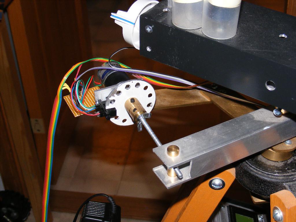
You can see the motor, the hole disc, the optical fork
(in black), the screw, a threaded joint in brass, and
the lever arm in aluminum.
This is the correspoinding arrangement in elevation.
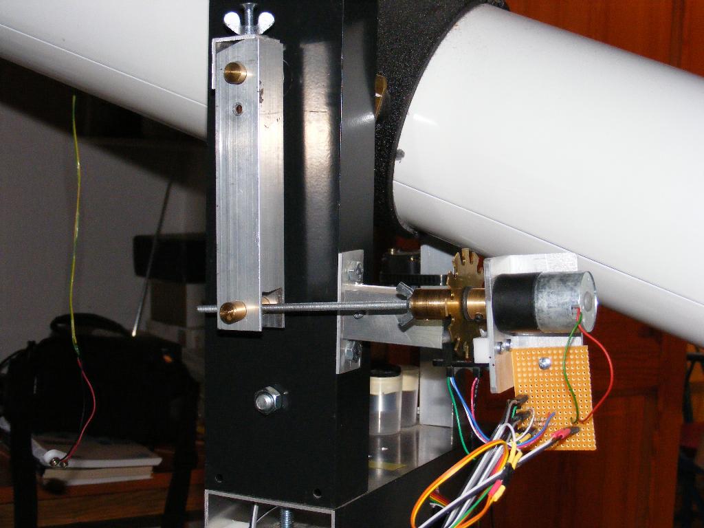
The
disc is slotted rather than a hole disc, which makes the
mechanical mounting of the optical fork a little easier.
You can also see the arrangement that locks the lever
arm to the elevation axis of the tube, with its wing nut.
Inside the aluminum tube profile, there is piece of brass
with an oval hole, which is pressed towards the elevation
axis.
It is worthwhile also to have an electric focusing. If
not, you have to touch the oscilloscope focusing knobs,
and it is hard to make the gimal arrangement so stable,
that it doesn't shake a little. Focusing is something you
have to do, after you have changed ocular. Fortunately
I have two amplifiers left for driving a focus motor,
and i have two buttons left on the remote control. The
software is simple, but of course you have to find out
how to couple a motor to the focusing knobs. This
picture shows how I have done it:
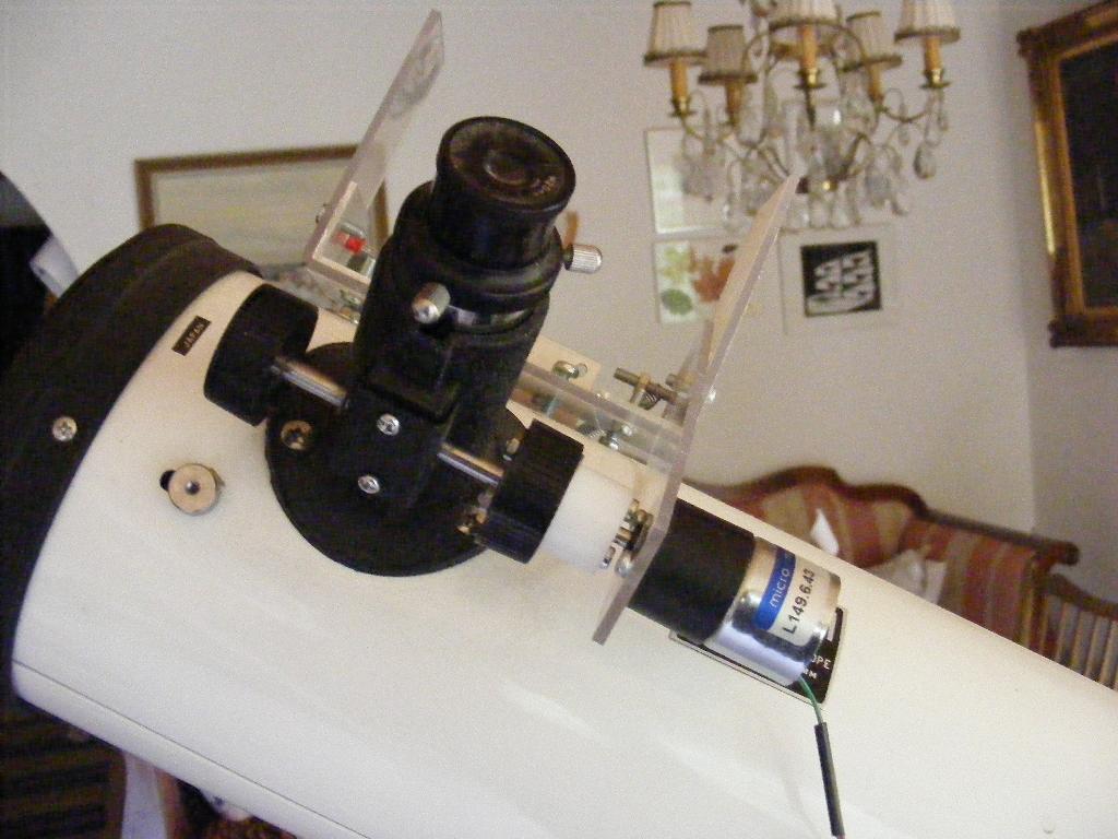
The computer has four input signals. Azimuth and elevation
signals come from potentiometers. They are right now handled
manually. The user is supposed to direct the elevation
potentiometer parallell to the telescope tube. A link arm
could make this automatic. The user is supposed to direct
a bar fixed to the other potentiometer to the south. An
electronic compass could do this, provided it would be
calibrated. The other two signals come from the optical
forks. All these signals are fed to the A/D converter.
The output from the computer is three pairs of motor signals
connected to the two poles of the three motors through
power amplifiers. These amplifiers are the integrated
drivers mentioned here. As
mentioned, the integrated circuits are mounted together
with protection diodes and a 5v stabilizer on little
modules. Each module can drive two motors, so to drive
6, I need two modules.
Now, we think of motor control as setting a six bit code,
which controls all three motors.
A code of 101010 would drive all three motors forward.
A code of 000100 would hold the first and third motor and drive
the second motor backward etc. The toggle process
sets these codes based on the state variables xel an xaz,
and the fork positions. In turn, these computations rely
on the time intervals dtel and dtaz, and on the directions
direl and diraz.
The process motor sends the code further to the
amplifiers, which amounts to shifting the codes to the
right pins, and clocking the shift register. It also has
to satisfy the amplifiers requirements to get zero input
now and then.
The times dtaz and dtel and the directions diraz and direl
are computed by the times process, which contains
the table from the Java program. In fact dtaz and diraz
are constant. The computation of dtel is based on a table,
where azimuth and elevation have been discretized to
tens of degrees.
This discretization is made in the anal process
together with the A/D conversions. The discretization of
the elevation angle is based on measurements. The optical
forkpin signal are discetized to boolean values, using the
G assembler function, which maps any number greater than
0 to boolean true (1) and any other number to boolean false
(0).
Finally, there is a manual control of the telescope from
the standard remote control used for the robot. The remote
control signal
is received through Proto Zigbee and is called comm. It is
a mapping of the buttons pressed, and it requires that
only one button is pressed at a time. The manual
process computes motor codes similar to those from
the toggle process, and they also control the focus motor.
If no elevation button (the upper and
lower) are pressed, an ignore code is set. Similarly the
azimuth motor code and the focus motor code can be set
to ignore. The merging of
the "automatic" motor codes codeel and codeaz, and the
manual ones, mcodeel and mcodeaz is done in the process
toggle. If a manual code is not ignore, then it overrides
the automatic code.
Download Teleskop.mps
Download Display.mpo
Download Telskop.java
Download Text.java
(used by Teleskop.java)
Here is finally a short manual to the telescope:
- Make sure that the lever arm threaded joints
are in appropriate positions along their screws.
The azimuth joint could be towards the end of the
screw (It will move inwards).
The elevation joint could be near the middle
of the screw. Arrange this with the remote control.
- If you feel you want a cup of coffee, or expect
that the next step will take some time, disconnect
the power to the electronics.
- Loosen the gimbals from the lever arms.
In elevation you could see a wing nut for
that in one of the pictures above. There is a
similar wing nut for the azimuth.
- Direct the telescope tube to what you want
to look at using the manual sight on the
tube. When ready, tighten the lever ams to
the gimbals again.
- Align the elevation potentiometer along the
telescope tube, and direct the bar on the
azimuth potentiometer towards south.
- Reconnect the power to the electonics.
- Look in the telescope ocular, and if you
see your astronomic object there, center it
with the remote control. Otherwise you have
to scan around with the remote control to
try to find it. This can be quite difficult,
so you may prefer to go back and use the
sight on the tube instead.
- Once the object is in the center, it will
stay there for a good while. You may have
to adjust after a while with the remote control.
- Now you can also start changing ocular to
get a closer look, and you can do that without
having to worry where the object goes while
you don't observe it. It stays where it is.
- After more than a good while, you will have
run out of threading of your screws. No more
to do than to go back to point 1 again.
The Digital Camera
A commercial digital camera is an impressive thing.
It has an image sensor that gives something from 0.5 Mpixel
to 12 Mpixels. Then it has a display with maybe
1 MPixel, and there is electronics that transfers the
pixels between the two
so that you can see the image in real time. That calls for
an update rate of at least 20 Hz. 1 MPixel in color is at
least 2 MBytes (16 bits per pixel in color information). So
we have a data rate of at least 40 MBytes per second.
That is far more than you can achieve with standard serial
protocols. And it is not only to transfer the bits; you have
to get them out from the camera sensor and into the
graphical display. Furthermore, there is the JPEG
encoding of the pictures, which is far from trivial.
If we would like to do something as amateurs, the best thing
is probably to get some sort of camera sensor
with a standard RS232 or SPI output. That means that the
manufacturer of that sensor has solved most of the problems
for us. But it gives us a camera, which we can use for
things like robotics applications.
There used to be such a camera called C328. It had an auto
baud rate detection, which could maybe be nice, but I never
got it to work reliably. The newer version is called C329,
and it works better. I still have some difficulties syncing
the data, so I have a special fix for that.
A somewhat odd alternative is the latest version of
the CMUcam, developed by Carnegie Mellon University.
This version uses a Propeller processor, but it seems to be
a missuse of a Propeller. The point is, that, like all
microprocessors, the Propeller has far from enough memory
to store a whole picture. The solution would be an external
RAM. But CMU's solution is to download the entire picture
several times, and screen out a single row each time.
This gives an exposure time of a picture of 3 seconds (!)
of more.
Back to the C329! It comes in two versions, RS232 or
SPI. Probably it is a good idea to buy the SPI version,
but I didn't! The point is, that with SPI, the master, which
is the Propeller, controls the clock pulses, and can thus
get itself the data at a rate, that it can handle. With the
RS232 alternative, the camera pushes the data, and
there is always the risk, that the Propeller is flooded
with data. This rules out direct writing into SD-cards. While
the SD-card shifts write page, data are unavoidably lost.
So with the RS232 camera, data have to go to the RAM
first.
The C329, like the C328 can send you a JPEG encoded
(compressed) picture,
which is nice, if you just want to send your image to a
PC, which has facilities to make JPEG decoding. But
JPEG decoding in a microprocessor, like a Propeller, seems
to be an overcourse.
For the uncompressed image, you first
have to choose a color format. My choice is the 16 bit
format (two bytes per pixel) where red green and blue take
up 5, 6 and 5 bits respectively. Then we get "files" with
two bytes per pixel.
The "camera" comes as a breakout board with an optical
sensor and electronics, but the lens has to be ordered
separately. There is a lens holder which fits to the
breakout board. But the threading of the lens or the
holder was so poor, that I needed to make my own lens
mounting. The threading of the lens is very fine grained,
so I didn't think I could make such a threading, so
instead I mounted the lens in an O-ring, which worked
as lens holder.Then the whole thing was mounted in a
little box.
Here's the camera mounted on a "Gorilla pod":
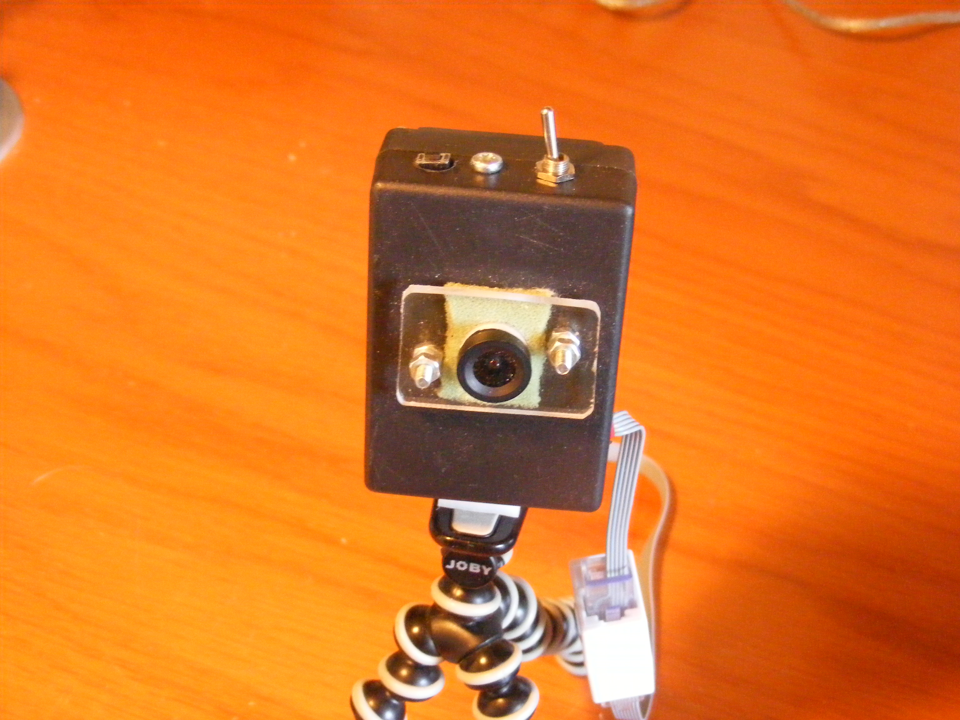
The system now consists of the following: The camera and
its lens, a Propeller, the RAM, an SD-card and a keyboard
for control of the system, and the RGB-led. When turning
on the system, there will be an initialisation of the
camera. Unfortunately, before doing the initialisation, the
camera has to have its power off. Then, the successfull
initialisation will be signalled with a green LED signal.
Then, when the operator hits the enter key on the
keyboard, a picture will be taken and will be stored
in the RAM, and then displayed.
Now to the mysteries. The camera sends some data before
the actual picture. Many data. It seems to vary a little
too, and I haven't found out how that works. Safest is to
put everything into the RAM. If the numbers of bytes is
odd, the color bytes will change place, so the colors look
really odd. To get it right, I shift the adress to the
RAM a little, under control of the keyboard. In that way,
by displaying the picture a couple of times with different
shift, I can get a nice picture.
Then I'm almost ready to store the picture on the SD-card.
But to do this, I first have to choose a place on the card.
As mentioned, I don't have a file system on the SD-card,
so I have to choose an adress space manually, again with
the keyboard. Then I store the picture, and the RGB-led
shows again, when the storing is done. Then I can use
the picture display program, presented next, to show the
picture. And it is possible to write a program that uploads
the picture to a PC.
Here now some information about initialisation of the
camera. This is done by means of the cam.mpo
object file.
The camera wakes up with an expected baud rate
of 14400. We will change that to 155200, but it we want
to initialize the camera again, we have to bring it back
to 14400 by removing power. Then the first to do is a
syncronisation procecure. This is done with a sync command.
All commands
start with $FF $FF $FF (three bytes with only 1:s). Then
follows the command number in one byte,
and 4 bytes with parameters. Unused parameters are coded
with 0.
The sync command has number 13 ($0D) and no parameter.
The receiver of such a sync command is supposed to
respond with an acknowledge command. This has number
14 ($0E) and the first parameter is the number of the
command responded to. So we expect that response from
the camera ($FF FF FF 0E 0D 00 00 00). We wait for it 25 msec, and then
we give up, and try again, and we do that for a maximum
of 200 times. The administration of the waiting i done
in the function cam.wack. Now when sync is hopefully
successfull, the camera will send a sync command to us,
and we should respond to that with a $FF FF FF 0E 0D 00 00 00.
Then it is time to set the camera parameters. This is done
with command number 1 and the following parameters:
- Baud rate. 7 is 14400, and 4 is 115200. These are
the ones I use, but it is possible to go up to
921600, which has code 1.
- Colour type. Code 6 gives me what I want, i.e.
the colour information is encoded into 16
bits (2 Bytes) with 5, 6 and 5 bits for red, green
and blue.
- Preview resoution. Code 3 gives me
160 x 120. Not terribly much, but it is what my
display can handle. 5 gives 320 x 240.
7 gives 640 x 480.
- Compressed image resolution. The codes are
the same as for the preview. I'm not going to
fetch any compressed images, but 0 might be offensive,
so I use 3.
Now the camera is ready, and we can get a picture by
sending a get command. The command code is 4, and
the first parameter is 2 for getting the preview image,
i.e. an image with the resolution set above. The bytes
come flying now, and we grab them with the cam.grab
which we start in its own process.
Furthermore, cam.mpo contains the following functions:
- cam.display for sending the image directly
from the camera to the display
- cam.toram to send the image to the RAM.
- cam.ramtopc to send the RAM content to the
PC (one image size).
- cam.ramdisp to send the image in RAM to
the display.
- other stuff, like synthetic images and some
experiments with image processing.
Some of these functions use the cam.read function
which has a timeout function to detect, that the whole
image has been sent.
Here's a picture of the whole setup:
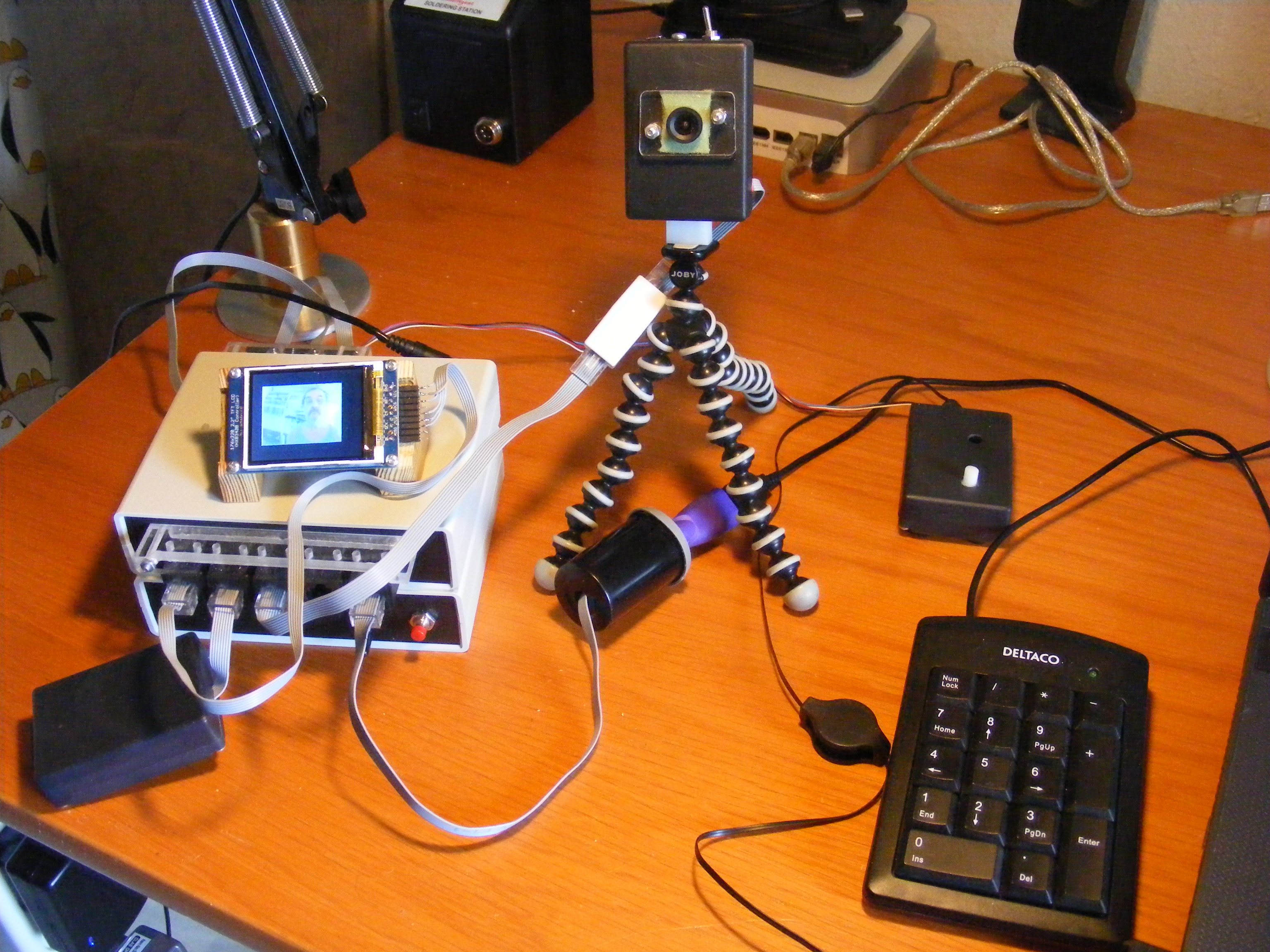
These are the functions of the buttons at the keyboard:
- Enter, takes a picture, stores it in RAM
and shows it on the display.
- Del redisplays the picture
- 5 shifts the output from the RAM one step.
This should correct for if the colors are false.
Type Del to see the result.
- 4 moves the picture to the left, one pixel
for each press. Check the result with Del.
- 5 moves the picture to the right.
- 9 will increase the SD-card block number
with one. When this button or button 3 is
pressed for the first time, the SD-card block
number will be displayed on the display. There
is no account in the computer for which blocks
are used, so you have to keep track of that
yourself (place for improvement).
- 3 decreases the SD-card block number.
- + stores the picture on the SD-card. This
takes a little while. In the meanwhile, the RGB
LED will show magenta.
When restarting the computer, the RGB LED will first
show yellow, and then hopefully green. If it shows red,
a reason might be, that you have restarted the computer
without restarting the camera. Turn the switch on the
camera off and on, and then restart the computer.
Here are files to download:
cam.mps
cam.mpo
ram.mpo
morse.mpo
sdh.mpo
key.mpo
grafa.mpo
col.mpo
Picture Shower
So far, this program is a little bit scetchy, but it allows
you to look att pictures stored on an SD-card. So far, the
program only uses single hits on the keyboard, which controls
the showing. Hence the number of pictures to show is limited
to 16. The pictures shown are of three different formats,
and the encoding of which format each picture has is put
directly into the program. So improvements are possible.
The three formats are the following:
- A format from pictures fetched from the PC.
They have the same resolution as the display;
220 x 176 pixels, and they are stored row by
row. The Java program that generates these
pictures fill with black up and down or right and left
to maintain the proportions of the pictures.
- A format for pictures from the CMU-cam, from which
I have a few pictures. The size of the pictures
is 160 x 120. Every pixel is stored in two bytes
and there are no "padding zeroes" on the SD-card.
The pixels are stored row by row.
- A format for pictures from the C329 camera.
The size of the pictures is the same as for CMU-cam,
put the pixels are stored collum by collum, which
requries some extra programming.
The procedure for getting the pictures from the PC
is this. The Java program ToFile.java generates files
from the pictures. The program name is of course a little
cryptical, but it resides in a directory for Photo processing,
which perhaps makes it more understandable. The program is
also quite primitive. You have to go into it and write
input and output filenames manually.
The files generated
are simple accounts for the pixels of the image.
The color information for each pixel takes up two bytes..
These bytes for a pixel are stored in text format
style, with each byte represented with hexadecimal characters
encoded in ASCII. This file format is called .hmp.
(that is my name for it).
Then these .hmp-files are transferred to the SD-card
through the cooperation of one Java program, Imsend.java,
and one MPS-program, StoreH.mps, sitting on either side
of the "PC-umbillical" to the Propeller. ImSend converts
the hexadecimal representation back to plain bytes, and
these are then stored on the SD-card. As we regard
the SD-card as a memory of longwords, these bytes are
stored in groups of 4 bytes. ImSend.java waits for
a request from StoreH.mps in form of an arbitrary charactes,
So you should start ImSend.java before StoreH.mps. Having
run these programs, you have your picture in the SD-card
ready to show.
The program in PictureH.mps uses 4 parallel processes.
One (keyscan) just reads the keyboard. One
(keychoose) reacts
on the outputs from the keyboard and sets an SD-card block
to read from. These blocks have the size of 215
bytes. Once a block has been chosen, keychoose resets
semaphores, so that the memory and the display are
reinitialized. Then the process get gets data from
the SD-card, and writes it into the variable data,
and the show reads data from there. This traffic
is controlle by the variable hasdata.
Both get and show are split to different
routines for the different image formats. Some of these
differences depend on differences between the formats,
that are maybe a bit arbitrary. The main difference between
showcmu and showc329 is that the pixels are
stored row by row and collum by collum in the different
formats.
Here's an example, which is also a self portrait of the
author:
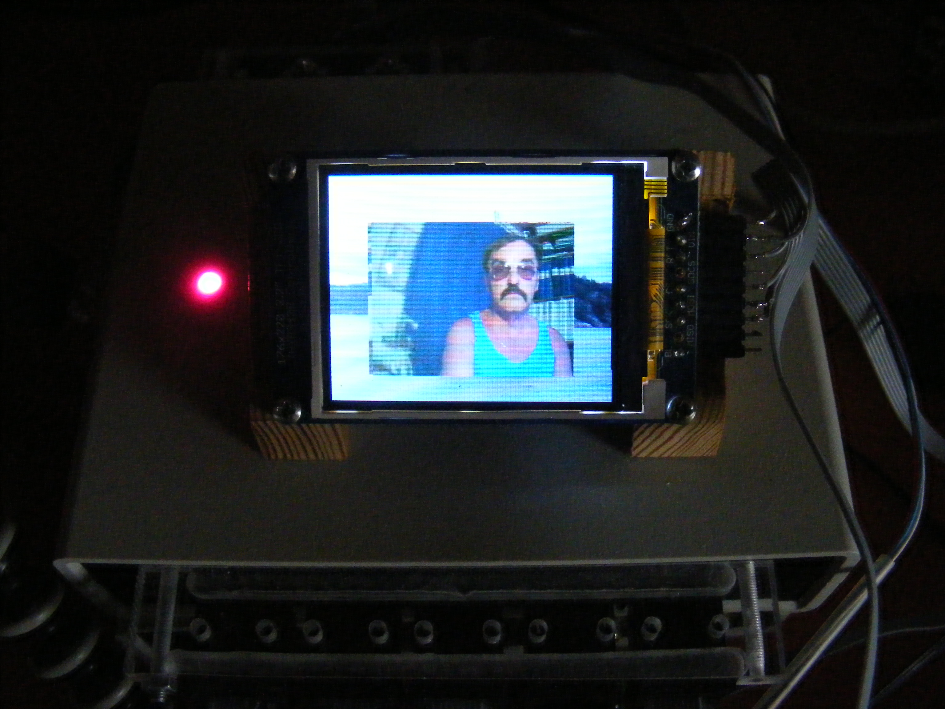
The FM Radio
This radio is based on a chip from Airoha called AR1010.
In a volume of 4x4x1 mm3 it contains a complete FM radio
with stereo decoder, sound outputs and two different
computer interfaces. I don't know if this is a so called
Software Defined Radio, i.e. a completely computerized
radio, or if there are any special circuits. Nevertheless,
you don't see any traditional things like coils or capacitors.
My work is based on a small breakout board, which includes
a crystal. It is sold by Spark Fun Electronics. Apparently
Telefunken has made circuits of this type, and there is
another chip called SI4375. Read about that
here.
The problem with Airoha AR1010 is that the documentation
to it is confidential! All that is availble is a
datasheet that describes the electrical connections, but
it says nothing about the protocols, with which you speak
to your radio chip. A software specification is avaiable on
the internet, however,
though it is pretty hard to find. The name of the document
is ar1000F_progguide-0.81.pdf, which you can try on Google.
One adress you find is www.docin.com/p-34190202.html which
is a chinese site where you can see and read the document,
but it is unclear to me how to download it. I have downloaded
the document, of course, but I don't dare to make it
available here. Some people have complained about the
quality of this document, but I think it is quite good.
As you can see from the name, it is actually about the
circuit ar1000, which is a more advanced sister to ar1010,
which has RDS, but it works for ar1010 also.
The breakout board is maybe intended for surface mounting
on a circuit board, but it is easy to connect to a normal
hole mount board with some small wires. The breakout board
hides some details of the original cicuit, so all you
have to think about is this:
- Ground and Power supply (2.5 - 3.6 Volt)
- Antenna input
- Sound output (2 stereo channels)
- Four connections for interface to the
controlling computer.
If you ground the Busmode pin in the computer interface,
you get I2C interface, and then all that remains
is a clock pin and a data pin. We have mentioned about
the I2C interface here and
here will come some more detailed information.
The AR1010 chip has 18 registers, each with 16 bits, and
you control the radio by writing into these. The procedure for
this is the following:
- Send an I2C start pattern
- Send the adress of the chip, which is
hexadecimal 10, but this should be followed
by a 0 write bit, so what you send is actually
hexadecimal 20 (in one byte)
- Send the number of the register, you want to
write to.
- Send two bytes of data, to fill the sixteen
bits of the register.
- Send an I2C stop pattern
All this can be done with the iic.mpo object file.
With a similar pattern
as above, you can also read any register, to find out
about the status of the radio. I found that unnecessary.
I trust that the radio will do what I tell it, and I
expect that the corresponding status bits will be set, if
I just wait a while.
The programming guide describes the contents of most of
the registers, but it is obviously an incomplete description.
There is a set of default settings to all the registers, and
sometimes you set bits to registers that, according to
the description, don't mean anything. Anyway, the default
settings work fine. There is one set of default settings
if you have a crystal on the chip, and another if you set
the reference frequency from your computer, but here we
do have a crystal. To initialize the radio you should set
these defaults from register 1 and up, and last to register
number 0. You will find the default values, and how
to initialize the radio in the file radio.mpo.
The rest of the settings have to do with setting frequency,
setting volume, muting and unmuting.
Radio.setfreq receives the frequency in 10:ths of MHz. This
is also how the frequencies are distributed to the users.
If you want to transmit something on the FM band, you are
assigned a frequency in MHz with one decimal. So if you
hit that frequency in the receiver,
which you should be able to with
a crystal, you should be exactly tuned. If you multiply
the frequency with 10, to get an integer, and subtract
690, you get something called a channel number.
That channel
number should go into register 2. You first write into a
mirror of that register in the computer, and
then send that mirror over to the real register. But
you also have to toggle a so called tune code. The
radio retunes, when the tune bit switches from 0 to 1.
Previously I muted the radio during the frequency switch,
but it doesn't seem to make any difference.
Volume is set in radio.setvol which receives a
volume number between 0 and 15. For some reason, the volume
scale is turned up side down, so you should send
(15 - volume) to the radio. This volume should be sent to
register 3. There are some less significant bits for volume
in another register. The programming guide shows how you
could use these bits to get a smooth scale, but I thought
that 15 steps of volume is enough, so I skipped the other
register. The 4 bits of volume information should be shifted
up seven steps into the register. But register 3 contains
other information too, so you have to mask it a little
to save the rest of the information in the register.
I chose to use potentiometers as input to the radio. They
are A/D converted, and discretized to a number between
1 and 15 for volume and 1 and n for frequency, or rather
station, where n is the number of stations I'm interested
in. Then I have table for the frequencies of these stations.
Somehow you can find frequencies for your favorite stations
over the Internet. This is found in the main program in
the file Radio.mps.
An aspect on this, is that when you move with the radio,
you have to reprogram it, to feed in new frequencies.
I do that twice every year, as I move to and fro the
countryside. You can do things otherwise. You can vary
the frequency continously, and display the frequency
on an LCD-display, or you can use the chip's built in
search facilities.
The Propeller with it's EEPROM, crystal and voltage
stabilizers is placed in a box together with the radio
chip itself, A/D-converters (for the control potentiometers)
and pull up resistors for the I2C-bus. There
is also a RGB-LED to indicate the current choice of
station.
I was a little concerned about putting a 69 to 108 MHz
radio together with a computer with a clock frequency
of 80MHz, but it doesn't seem to be a problem.
The box is hung up between two PC-loudspeakers. I use
the audio amplifiers there of course, and I have also
broken myself into the box, to bring out 18 volts of
power to drive the circuits. It turns out that the
3.3volt stabilizer doesn't heat up, despite the relatively
high input voltage.
On the top of the box, there is an aluminum sheet, which
serves as a ground plane for the antenna, which in itself
is a metal rod, attached by means of a piece of plastic.
The ground plane is connected to a wire, which is clamped
on the outside of the power cable. For the 100MHz
signals, this gives some connection to ground, but the
50Hz power signal can't penetrate the small capacitance
between the wire and the power cable. This arrangement
helps improve sound quality, when the reception conditions
are bad. In my home they often are.
But the exact tuning, and the good sound quality of
the radio chip, makes this an excellent radio.
Here is a picture of my radio:
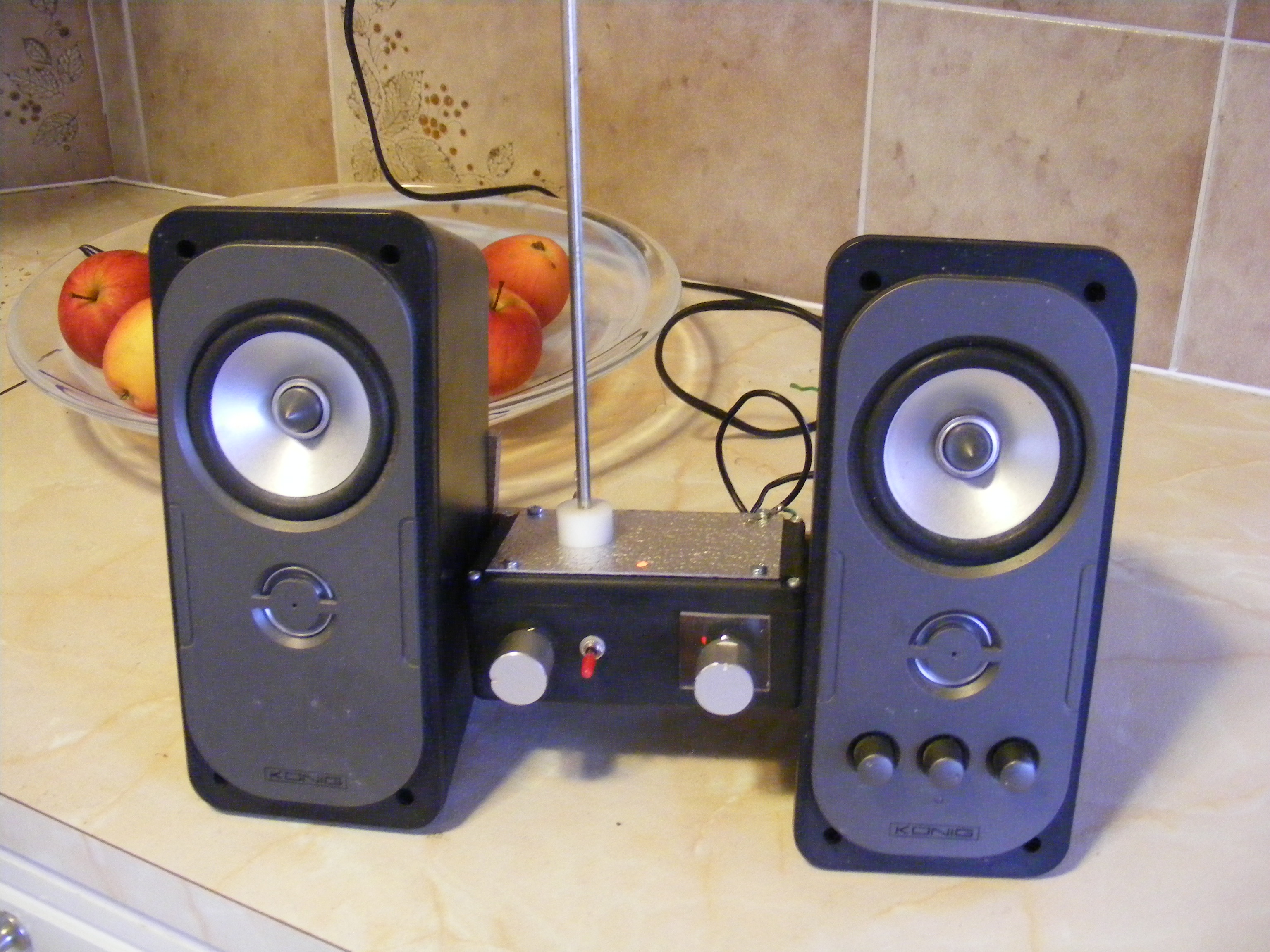
Download radio.mpo
Download radio.mps
Download iic.mpo
The Si4703 Chip
The Si4703 radio chip is an alternative to AR1010, and
it is maybe more accessible than AR1010 nowadays. It comes
on a breakout board from Spark Fun, which contains
a radio chip, a few discrete components, including a crystal,
an earphone amplifier and plug, and connections to a computer.
Programming Si4703 is about as confusing and difficult as
programming AR1010. There is example code to fetch from
Spark Fun written for Arduino by Nathan Seidle.
But Arduino has I2C communication
built in, while with a Propeller, we have to do it ourselves.
But, we have already done that. Also I think that the
Nathan Seidle has overdone some things a little.
Apart from the example code, there is a data sheet, and
a programming manual. The programming manual is OK, but it
has to be read together with the data sheet. The necessary
information is spread somewhat randomly between the two
documents.
The device can be controlled with two communcation protocols.
One of them is clearly I2C, but this is never
mentioned, so it's called "2-wire interface". There is a
reset pin, that you bring down for reset. When you lift it
again, certain states have to be present, to take the system
to the 2-wire interface mode. There is an inverted SEN-bit,
which has to be high, which it is on the breakout board thanks
to a pull up resistor. Then the SDA bit (in I2C
terminology; it is called SDIO on the board) has to be low.
Finally a GPIO3 has to be low. That's a bit bothersome,
becaulse that pin is also a part of a crystal oscillator.
But, be calm, It is low. So bring the reset pin down,
the SDIO pin down, and then lift the reset pin. Then the
device wakes up in I2C mode, and we can start
I2C on our side by calling iic.init from
Iic.mpo.
As is usually the case, I2C devices are handled
by writing to and reading from a couple of registers, in this
case 16. But they are written and read in an unusual way.
The device has default register addresses
for reading and writing. It starts there, and then
it increments its adress counter for every 2 bytes. It's
comfortable, but it means that you can't write to a single
register without writing to a couple of others too.
For some reason I failed in programming a register read
function. It reads all right, but it somehow destroys the
register contents. Nathan Seidle advices
us never to write to registers without reading them first.
The data sheet gives you the same message. But the programming
manual says: "The data sheet tells you what the registers
contain, and you can trust that, so it is not necessary to
read the registers." So, I accepted that, and it made the
whole task a lot simpler.
Now we come to the mysterious register 7. The first bit of
this register controls the crystal oscillator. You want that,
so you would like to write that register. The programming
manual says: "Write hexadecimal 8100 there". Then the first
bit is set, as wanted, and another bit for some unknown
reason. While we write register 7 we have to write all
registers from 2 to 7, but it's OK to write 0 to all of them.
Now, the crystal oscillator wakes up, and we should give
it about half a second to stabilize.
Now, the device is in power down mode, so we have to lift
it to power up mode. We do so, by setting the last bit
in register 2 to one. It is called Power enable. For some
reason they want us to set the next highest bit too, so
we do that by writing hexadecimal 4001.
While we do that, we can write to the rest of the registers
too. Register 2 to 7 are writeable. Most bits in these
registers are set to default values, that serve us well,
but, at least, if we are Europeans, we have to adjust a
few things. To reduce noise, the transmitters send
the higher frequencies of the sound with higher gain, and
you should compensate this in the receiver. This is
called deemphasis, and there is a special bit for setting
European deemphasis, while the default is for American
deemphasis. The UHF band is different in Japan on one side,
and America and Europe on the other. The American European
standard is default, so we don't need to change anything.
Then there is the channel separation, which is 0,1MHz in
Europe and 0.2MHz in America, so I have to deviate from
the default there. That's about all. Setting of frequency
and volume, will happen later.
Now the radio is powered up. In 110 ms it is ready to use.
For some reason, the mysterious register 7 now changes
from 8100 to BC04, but that happens by itself. So no worry,
but you shouldn't set the register to BC04 directly. Then
the radio doesn't work.
All this is the content of the function radio.init
in radios.mpo. It uses its own function
radio.writeregs and various function from
iic.mpo.
Then volume is set by writing the four LSB's of register
5.
Setting frequency is only slightly more complicated. First
we have to convert frequencys to channel number. If we
give frequency in the unusual sort of dMHz, which gives
us all frequencies as integers, we only need to subract
the UHF-band-bottom frequency, which is 875 dMHz, to get
the channel. We write that to the LSB's of register 3,
where we also write the first bit to one. That will trigger
the tuning in the radio. Then we have to wait for the
radio to react, and then we send the same information
again, but with the tuning bit reset.
Here's the code for download:
As you can see, I haven't bothered about RDS, Radio Data
System, which gives you information about the programs.
The Media Player
I won't give all the details of this application, which
is a media player, which can play radio, MP3-files
and TV sound through full size loudspeakers. Here's
what it looks like:
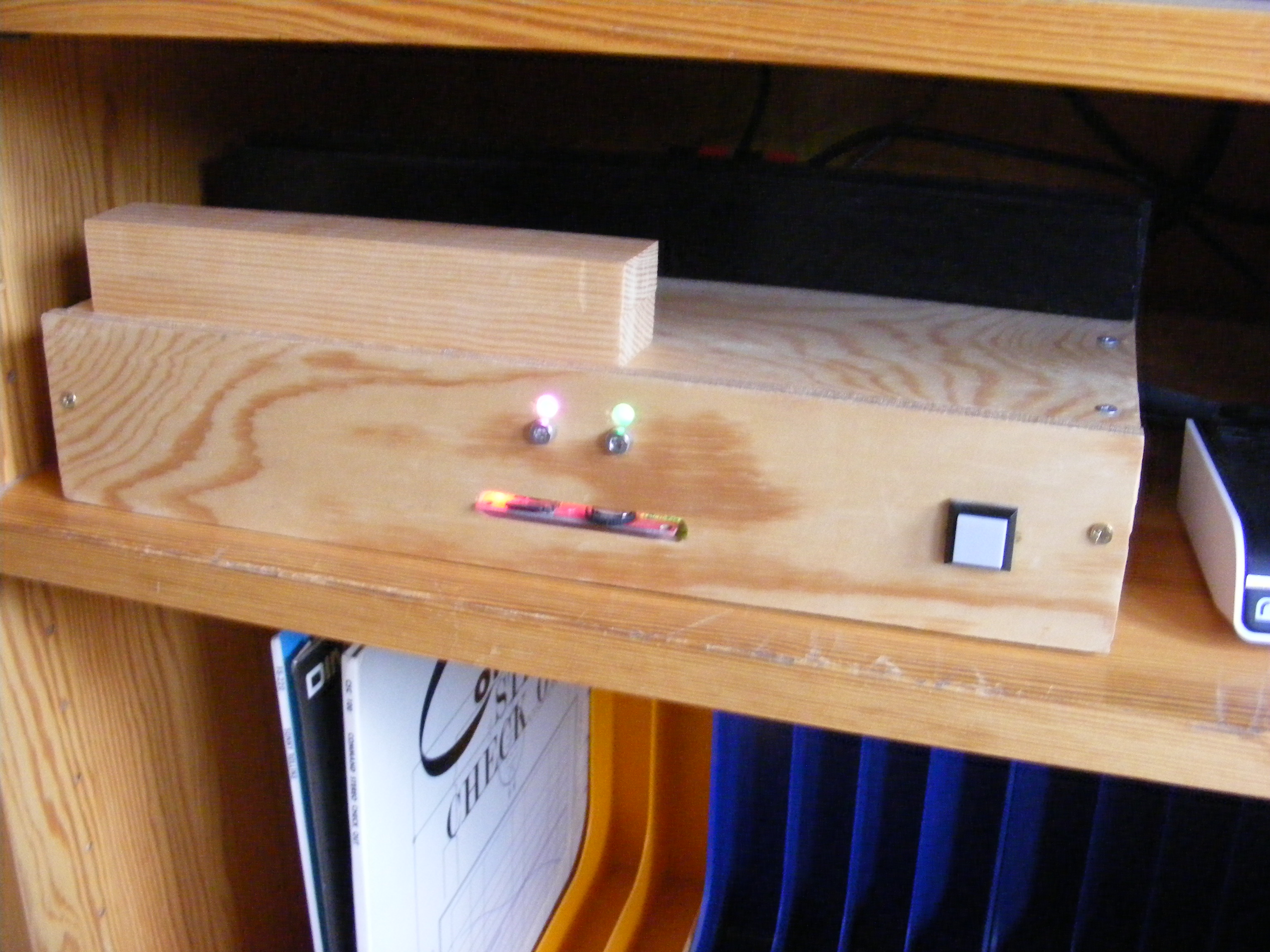
As you can see, there are no knobs and buttons on the
device, except a power switch to the right. Instead it
is controlled entirely from a remote control. To see
what you have done, there are two RGB-LED's. You can
also see the MP3-player through a slot. I had to put it
that way, so that the micro-SD-cards, that contain the
music, could be pushed in. The back part of the box is
a little higher, and black, so you don't see it (do you?).
It contains the power supply and the cooling element
for the power amplifiers. On top of the box, there is a
smaller box, that contains the micro-SD-cards. They contain
the content of a heap of vinyl LP-records, that is about
2 meters high.
Here's the remote controller:
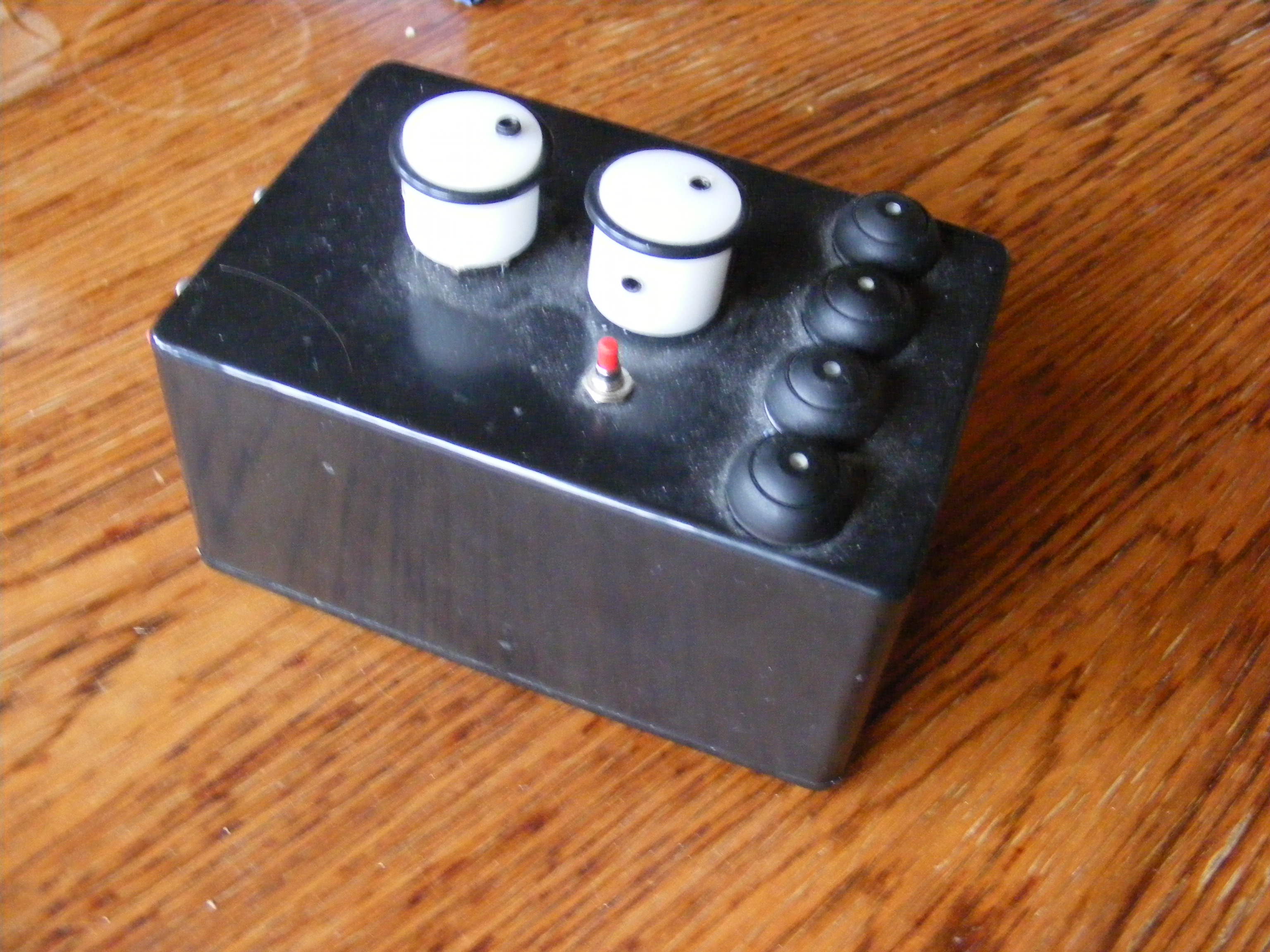
It communicates with the player over proto ZigBee. It
has two knobs, one for volume, and one for selecting
MP3 files. And four buttons for choice of Radio, MP3,
TV or nothing. And there is a power switch, to save
batteries. It consumes pretty much.
The control computer in the player is, of course, a
Propeller.
The radio is AR1010 as in the previous section. The
way this device is placed, there is a better antenna.
The MP3 player is a little board, sold by Spark Fun
Electronics (and resold in Sweden by Lawicel). The
music is loaded in micro-SD-cards on files with standardized
names TRKxxx.MP3. You choose file number xxx by sending a
command over RS232 to the board, and then the board
plays the music. There may be many of these boards around.
Choose one that let's you control it from a computer.
Then we make the whole thing electrically controllable
by using analog electronic multiplexers and electronic
volume controls.
The electronic multiplexer has the designation CD4051.
It may not be easily available any more, but some sort
of electronic multiplexers should be available also today.
More correctly put, these circuits are called analog
multiplexers, and they consist of analog switches. An
analog switch is a digitally controlled switch. with
either a low or high impedance from an input pin to an
output pin. By the way, the device is symmetric, so you
can swap the input with the output as you like. As long
as the signal that goes through the switch is well away
from the supply rails, the switch has a low resistance
in the on state. There is some resistance, and it varies
with the input voltage, but if you load the circuit with
high impedance, the on resistance is negligable, so
you can get an analog signal through with low distortion.
I supply the circuit with 12 volts, and to bring the
input signals away from the supply rails, I lift them
from ground with 6 vots from a voltage divider. That
DC component has to removed later on.
CD4051 has three adress inputs, and with them you can
choose between 8 different inputs going through to the
output. The control computer has to provide these three
adress inputs through 3 computer pins. So the computer
interface is "parallel".
The so called digital potentiometer, MCP41010, also has
analog switches. In fact it is a conventional chain of
resistors, as in "a discrete potentiometer", and analog
switches lead the signals out from some place along the
chain. The digital circuitry that handles these analog
switches is controlled over an SPI bus. (So now we have
a parallel interface for the multiplexer. SPI for the
volume control, I2C for the radio, and
RS232 for the MP3-player, and ZigBee unit, so it is a
good exercise in computer communication.) The digital
potentiometer has to be loaded with high impedance
to keep distortion down, so this section ends with an
operational amplifier OP290 in a follower configuration.
But the digital potentiometer, with its 10 kohms is good
as a high impedance load of the analog multiplexer.
The power amplifier is based on the TDA2050 power operational
amplifier as mentioned before. I use two for each channel.
One is configured as a non-inverting amplifer, and the other
as an inverting. Then I can connect the loudspeakers between
the outputs of the two amplifiers. That gives me twice the
range I can get with a single amplifier. Furthermore I can
adjust the two amplifiers, so that the difference between
the outputs is close to zero. Then I don't need any
output capacitors. But do this adjustment well! It is
said to be harmful for a loudspeaker to be driven with
DC current.
The voltage supply is a switched 12volt supply of the type
that is used for PC:s.
I enjoy this machine very much, and now I can play my
records pretty much effortlessly. No more carrying of
LP-records, and no more handling of pickups. Unfortunately,
by the time I built this, for some unknown reason, my
ears started working much worse than before, so I am not
the right person to judge the sound quality, but it's good
for me anyway.
GPS Logging
When I mention something about this application, some
people say: "I have it in my smartphone". Such are the
conditions for us "do it youselvers" nowadays. Everything
is already in the smartphones. What is the meaning of
life, then?
On the other hand: Doing the whole thing of GPS navigation
is hardly anything for us amateurs. There are a number of
satelites out there, and they send us their opinion of
time. When we compare these times from some different
satelites, we observe, that they don't coincide. But then
we have the theory that this lack of coincidence depends
on that it takes unequally long time for the time signal to
arrive to us from the satelites. With that, we can determine
differences in
distance to the different satelites. As satelites move
very regularly up in the empty space, we know where they
are, and then we know we, ourselves, are. Down to an error
of three meters or so! But that is not an easy computation!
Errors are a little bigger if we move in a forrest (or a
city) because the signals reach us after having bounced
a little between the leaves of the foilage. This growth
in error is quite fundamental, and there isn't much we
can do about it.
Let me say something about giving positions. The earth is
a ball. Then the surface of the earth would be a sphere
if the ball were perfect. How do you indicate position on
a sphere. Well, there would be many ways to do it, but
one of the best is to give longitude and lattitude.
First, then we would need a reference point. It is natural
to let that point lie on the equator. But where? Well, it
would be a point with longitude = 0. So where is longitude
0. Well, it's at the Greenwich Observatory, or at
Constantinople, at the Cheops Pyramide or in Paris. In fact,
for some time it was both in Paris and in Greenwich, but
finally the French had to give up.
The story continues this way: Someone placed a metal plate
at the Greenwich Observatory, and engraved a fine line in it.
That was where the zeroeth longitude went by. But then the
Americans made a radio navigation system, which pretty
quickly gained great popularity, and become a world
standard. It was not until after that, that someone came
up with the great idea, that one should place a receiver
at that engraved line at the Greenwich Observatory. The
receiver said "108 meters east (or west, I don't remember)
of Greenwich". So it was
wrong! But it was much more difficult to correct the
American Radio Navigation System, than to just move
the zeroeth longitude. So now it is 108 meters off
the Greenwich Observatory.
Then you move south along that zeroeth longitude point,
until you hit the equator. As long as we have the rotation
axis of the earth, that is actually well defined. The
point we find is the reference point. It has longitude
0 and latitude 0. We can imagine a ray going from the
center of the earth, out to the reference point. Then
we rotate that ray first around the earth rotation
axis, and then around an axis perpendicular to that, so
that the ray points at some given point. Then, the two
angles are longitude and latitude for that
given point.
Now, when the earth isn't spherical, we have choices.
The choice made has to do with so called Inertial
Navigation, which in aviation is often combined with
GPS. The result is, in practice, that these rays don't
start at the center of the earth. The key idea is,
that in each point on Earth, there is a plane (called the tangent
plane of the earth's surface) whose normal is vertical.
in the sense that it falls along the
gravity vector. To be precise, that vector gives
the direction of the sum of two forces: the gravity
and the centrifugal force, that comes from the Earth's
rotation.
The net effect is that, if we materialize that plane, a
ping pong ball put on it, wouldn't roll away, but stay
where it was. Now we have a z-axis as
the normal of the plane. We can fix one more axis, the
x-axis, by letting it point North, which means that it
points into the Earth rotation axis. Then the third axis
is given as an East axis. So this is the North East Down
system. It may seem unnatural to have one axis down, but
that is required to make the whole system a right oriented
system, which is desired. Now, we can make a similar system
in the reference point at the equator. Now the story is
to rotate the reference point coordinate system into the
local North-East-Down system. After we have done that, we
can make the two systems coincidence completely with a
translation, but we don't really care about that.
The longitude and latitude are now truly rotations.
This definition requires a model of the Earth. If the
earth is so irregular, that we couldn't hope to model it
as something "mathematical", we could still go along with
huge tables and the like, but it would be very complicated.
But luckily, the Earth can be modelled pretty well as
a so called ellipsioid. The German astronomer Bessel made
such a model in the 19th century, and up till a few years
ago it was a basis for the Swedish geometric system
called RT90 and its predecessor RT38 (Rikets Triangelnät 1938).
But then, when GPS was to be born, one found it worthwhile
to make av revision, and that lead to a new ellipsoid
Earth mode called WGS84. From that the geometric system
of Sweden has been revised to something called Sweref.
These geometric systems are about defined reference points
marked out in nature, and about map projections.
But the notions of longitude and
latitude are well defined, as soon as the ellipsoid model
is given.
The problem with the longitude and latitude is that we get a
very anonymous and long series of figures. A confusion is how
"Babylonian" we should be. Things like degrees and minutes
and seconds (arc seconds) are Babylonian in style, in that
one divides by 60, rather than by 10 and 100. The compromise
is that positions are given in degrees and minutes
with decimals.
All this is delivered with figures (and decimal points,
commas and the keywords E and N for East and North) encoded
in the Ascii format and delivered as RS232.
. This information is collected into
"messages" called GGA etc. These messages belong to a
standard called NMEA.
If you are connected with your Microprocessor to a GPS
receiver, which delivers these messages, you have some
work to do. One task is to throw out all messages you
are not interested in. I took the choice to pay
attention only to the GGA-messages.
A good GPS may deliver about
10 such messages per second. You may want to keep just one
message per 2 seconds. Then you might like to acquire some
data in numerical form, rather than as text strings.
One unfortunate property of the latitude longitude system
is, that differences in longitude (from one point to
another) are not comparable to differences in latitudes.
The longitudes run together as you approach the Poles.
We can see that in a commonly used map projection called
Mercator (from a Dutch merchant called Kramer, which means
merchant, and whose name was latinized to Mercator). It
just plots points on the Earth according to their
longitude and latitude, but to keep proportions intact,
the scaling in the northerly direction grows as you
approach the Poles. Hence you can never show the Poles
themselves. In such a projection, Greenland is about
as big as South America, while in reality, Greenland
is only as big as Venezuela and Colombia together. As
another example, Norway stretches in longitude from
Marseille in France to Alexandria in Egypt. Globally
we cannot do much about this. Whichever trick we try,
we loose something to gain something else.
But in a local neigborhood of some point, we can do
a linearization of the Earth's surface, which amounts to
working on the local tangent plane there. The trick is to
measure differences in latitude and longitude relative
to a reference point, and then
scale the differences in longitude with cosine of
latitude (This holds for a spherical Earth. For a true
ellipsoidic Earth it would be a lot more complicated
but no matter). At the same time, we could scale everything
to meters. For that, we convert the angles (longitude
and latitude) to radians, and then (after scaling of
the longitude) multiply by the Earth's radius, which is
approximately 6360 kilometers. With the format of the
GGA-messages, we get the angles as an integer that
represents the longitude and latitudes in 600000:ths of
a degree.
Right now, I have one such reference point in Sweden.
The data I get can be plotted, and the plot gives me
an image of my track, which is correct in directions and
proportions, and I can sum up my distance travelled.
So these positions is what I log in my on board memory
together with time in seconds since noon at Greenwich
that day, and together with the number of satelites
used. All this fits into 3 32 bit numbers, which I store
in a flash memory.
So here's in summary what the program has to do:
- Grab the bytes coming from the GPS receiver in
an RS232 form.
- Throw away everything that is not a message
of the GGA type. This is a message starting
with $GPGGA and ending when the next $-sign arrives.
- Count the number of GGA messages, and only keep
one per two seconds.
- Convert the time part of the GGA message
which is given in hours, minutes and seconds into
an integer representing all the seconds since noon in
Greenwich.
- Perhaps check for the characters N and E, so
that you are where you believe on the earth.
They could be S and W too. I don't care for this.
- Put the figures together with the decimal point
in the latitude and longitude information into
numbers representing the angles in 600000:ths of a
degree.
- Convert all this to positions relative to some
reference point somewhere near where you move about.
Above all this involves a scaling of longitude
differences with cos(latitude)
- Extract the number of satelites used by the
receiver from the GGA-message.
To store the data, I now use an EEPROM with 1 Mbits, and
a file system tied to it as described
here. I store 3 longwords of
data every 2 seconds, and then I can sample data for almost
6 hours. If that is not enough, you can decrase the
sampling rate further, or you can buy up to three more memory
chips.
I need a mechanism to generate an automatic file name.
It is done so that the page 2 of the EEPROM contains
an initial file name, namely "gp0". Every time the
Propeller starts, it takes this name, increments it with
one, writes it back, and then creates a file with that
name. There is a reset program that restores the name
to "gp0", when you think, the memory may be full.
Once the file has been created, and GPS position become
available, time and position data are written to that
file.
As a consequence, the files will be called 'gp1', 'gp2'
and so on.
If I get a power interrupt, when I'm out logging, I get
a new file. But I can paste that file and the previous
one together afterwards, to get a complete account for
my track.
Since I started to employ the EEPROMs for the logging,
this has worked very reliably.
We need the logging program of course. And we need the
reset program to clear the file catalog, and start over
from the file name "gp0". And we need a program to read
out the data from the flash memory.
You will find these programs in the next section
Downloads
This is the GPS logging program itself.
The file also contains some processes so that
you can verify functions over your PC. In the exec field
there are som different alternatives. The one calling
pcchar will show you the stream of data from
the GPS receiver. The one calling pcmess will
show you the GGA-messages at the rate you keep them.
The version calling pcpos will show you the
positions in meters. Use the program Propp.java for this.
(We will return to Propp.java in a while)
The version without comment marker (--) is the one
that loggs data.
You also have to modify the position function in
the evaluate process, to fit the system for the
place where you live.
It goes like this: Find yourself some good reference point
and determine its latitude and longitude. Google Earth
can serve you with this. Then you convert these angles
to 600000:ths of degrees. Put these numbers as la0
and lo0.
Then compute cosine of the latitude, using any pocket
calculator. We call that coslat. Then you compute the factor
1/600'000*pi/180*6.36E+06*coslat
The expression pi/180 is what it takes to go from
degrees to radians. 6.36E+06 is the radius of the Earth.
In my case this value is 0.0967723. Then multiply this
with 2^16 = 65536. That gives you an integer, which is
called sla. In my case that value is 6342
Then you need the following object files:
Furthermore you need these programs for resetting and
reading data from the device. They use the same object
files as above.
Some Java programs and instructions for use
The program gpsread.mps communicates with the
Java program Propp.java. It is presented
here. The program lets you
send and receive data to the PC. When data come
from the PC, they act as commands to GPSread, and
they make GPSread send responses to the PC. The
commands (that you type in the third textfield in
Propp.java:s window) are these:
- d is like the MSDOS dir-command. It sends over
all file names in the file catalog. Typically
they would be "gp1", "gp2", "gp3" etc.
- ngp2, as an example, selects the file
gp2
- c counts the number of pages (blocks, fragments)
of the file. It take a little while, but after it's
done a prompt, ">", will appear in window 1.
- s will then return the file size in pages
in hexadecimal notation. It is not very readable,
but what you really want to know, is that you
haven't found a very small file.
- g (for g) sends the whole content of that file
to the PC. In window 1 this content will seem as a
nonsense text, as it as interprets numerical data
as ASCII characters. You can avoid seeing this nonsense,
and the time it takes, as described below.
If the size of the file is not very small, or if you have
seen that nonsense text, you have found some navigation
data. To bring them to you PC for further processing,
do as follows:
Type s in the mode (4:th) window of Propp.java.
Then go back to the 3:rd window again, and type
g. Then the Propeller will send the
data again, but now they will be stored in an array
in Propp.java. Check with the LED on the Propstick to
see when the transfer is complete.
Next go to the mode
window again and type a filename followed by a
"<". Now you have rescued your
navigation data. It's easier in the sequel if
you give a file name that ends with .gps
Unfortunately
the USB communication can produce some undefined data
initially, so you have to go into the file with an
editor like Notepad to edit the file. The real traffic
starts after the hexadecimal characters AA. Remove AA
and everything before it. Then, in the end of the file,
there are some data, that may belong to a previous logg.
With some training, you can find a break in the pattern
on the file, at its end. Otherwise you can remove these
old data from the plot file generated later.
Using Google Earth
Then the perhaps most interesting thing to do with
your data is to plot them with Google Earth. For that
you need a GPX-file. GPX is a format which is a special
case of the XML format. The file contains data
strings, which describe longitude and latitude.
Isn't that sad? Didn't we just transform those data to
relative positions? Well, take it easy! The mapping we
used there is invertible, specially if we are less than
510 km away from the reference point. Look into the
position function in GPSLogg.mps. It's a fairly
simple linear function (as long as we don't have overflow).
Find out what the inverse mapping is and write into
the program GPXget.java (Download information
will follow)
There are instructive comments on how to do that in
the program. It just amounts to replacing some constants
to values that you have used in your GPSlogg.mps.
Now run GPXget with the filename witout '.gps'.
This will give you your GPX-file, which has the same name
but with '.gpx'.
Now start Google Earth, and open the open menu.
There is a choice to choose so called 'gps-files' If you
do that, your new gpx-file will appear. Double click on it
and answer OK to the next question. Then Google
Earth will zoom into the area where you travelled, and
show you trip.
Other uses
The program GPSget.java gives you a more straight
forward plotfile of your navigation data. Its name
is p[originalfilename].dat.
It's a readable
file, so you can look at how it is formatted in for example
Notepad. Then you can maybe find a plot program for that format
or a small revision of it. The plot will give you a
plot scaled in meters with correct proportions and directions,
if you manage to get the scaling in the two directions
equal.
To get even more interesting data, you could run the program
Dist.java. That will give you a similar file
called p[originalfilename]V.dat, and it will contain
two more variables: Distance travelled, and velocity.
If you walk, the velocity variable will seem very
noisy, but if you go downhill skiing, you can at least
see if you ski faster than you go skilifts.
Here's a picture from Google Earth:
This is a kayak tour around some islands at my sommer
place. I also made a slalom tour around the pylons of
a bridge. You can see how the track seems to be a few
meters east of the bridge. I also went up a bit into a
small creek. It may seem that I paddle on land a few times
but that's only because Google Earth has difficulties
in separating shallow water from land.
Java downloads
Here are the Java source file downloads
The latter three are utility classes that are needed for
all four programs. But Propp.java needs more. Refer to
this place for the details.
The Mandelbrot set
The Mandelbrot set is a set of complex numbers. Now,
as we have learnt here, a complex
number has two coordinates (the real and the imaginary), and
a point in the plane also has two coordinates, and thus
we can depict a set of complex numbers as a set of points
in the plane. So the set becomes a "figure" in the plane.
The Mandelbrot set was discovered by Bénoit Mandelbrot,
while he worked for IBM, but the Mandelbrot set has a
kind of dual relative, called the Julia set, discovered
by Gaston Julia and Pierre Fatou much earlier. But
Mandelbrot had the opportunity to make his set into
computer graphics, which quickly made it gain world
reputation.
The Mandelbrot set is generated from a very simple
equation (or rather function), but once it is there, and
you can show it with your computer graphics, and you can
zoom into its details, it reveals itself as an extremely
complicated structure.
Here is the function:
f(z) = z2 + c
z and c are complex numbers. What you do now, is
that you take what comes out of the function (f(z)) and
plug that back into z. And then you keep doing that. What
happens then? Well one of two things can happen, z can
stay limited, and maybe converge to something, or oscillate
in a limited world. Or, z can go to infinity. It depends
on what we start with, but we always start with z = (0,0)
= 0 + i·0 = 0. And it depends on the constant c.
Then, the Mandelbrot is the set of c-values, for which
z doesn't go to infinity.
To draw this, we start with some picture coordinates (ix,iy).
We map this with some linear mapping to a complex number
c = (cr,ci). Then we just run the
function iteration, and see what happens. We can't wait till
infinity for divergence, but the fact is that if divergence
happens, it happens pretty fast. Nevertheless, if we don't
wait long for divergence, then we miss some precision in our
drawing. OK, if there is no divergence, we draw a white dot at
our picture coordinates, and then we go somewhere else.
Here we wait for divergence 30 iterations. If z hasn't
diverged in these 30 iterations, we assume, that it never
will.
With this program we actually draw a three color figure.
We say that if z hasn't diverged after 10 iterations, we
draw it red, if not white. If it hasn't diverged after
5 iterations, we draw it blue, if not red or white. These
multicolored accounts for the Mandelbrot set became
quite popular after the publication of the Mandelbrot
set. But, it is the Mandelbrot set itself (the white area),
which is the most interesting.
The point now is, that by just changing the mapping from
(ix,iy) to c, we can effectively move around and zoom out
of and into the complex plane, and thus look for details
in the Mandelbrot set.
However, with fix point arithmetics, and 32 bits word length
(which is good enough for most purposes), it is hard to
give justice to the Mandelbrot set, so I recommend anybody
to repeat the experiment with, say, a Java program, where
the variables are represented as double precision floating
point values. In addition, you have a screen with higher
resolution.
But this Propeller program is a little feasability test,
which shows that you get a recognizeable Mandelbrot
set. Here's what it looks like with the Adafruit screen.
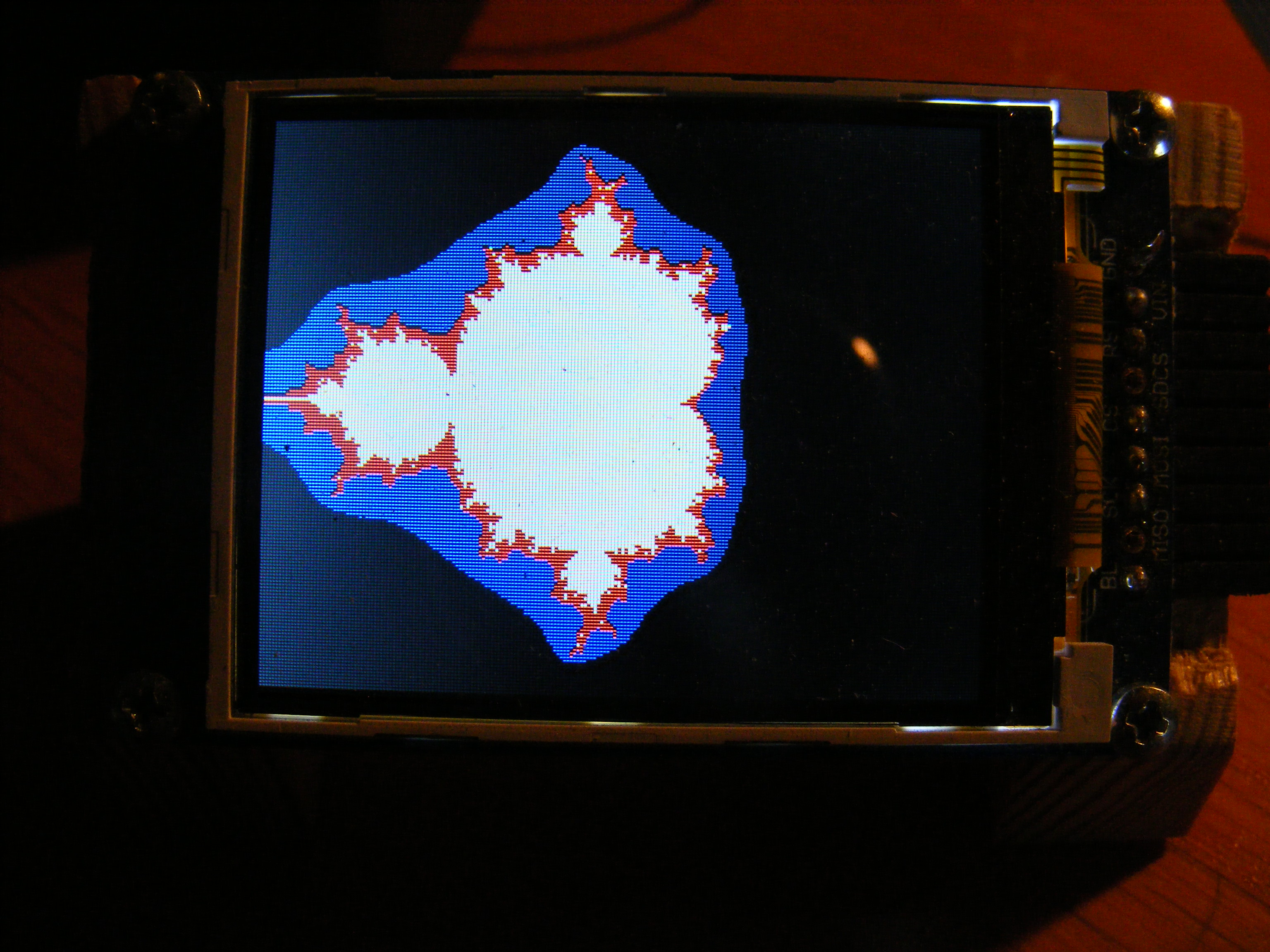
The limited resolution of both the display and the camera
gives the picutre a Moirée pattern, that you don't see
in real life.
Download Mandelbrot.mps
I hope you can follow the program from the code. It has
an outer loop over all the display pixels, and an inner loop
of iteration, which goes on for n=30 iterations, unless
there is a divergence. The pixels are generated in such an
order, that you can fill the pixels by just sending the
pixel color for each pixel.
Recent developements
Linux
After having spent lots of time on waiting for Windows
to start up, I decided to switch to Linux. I bought a
new computer with Linux Ubuntu installed. For the Propeller,
I installed a Linux Propeller environment. It works fine,
but I miss the possibility to run it from a command line
call. Always with Linux, one has to consider, that
Linux distinguishes between small and capital letters
in filenames, which creates a great deal of work.
USB has to treated a little differently in Linux. USB
has to be used, as serial communication goes over USB
in the so called Prop Plugs. In Windows, Java doesn't
have good support for USB, so you have to use C/C++ code
and so called ports. In Linux, they have the view, that
a USB port is a file, called /dev/ttyUSB0. This isn't
quite true, though. For a file, you have a program,
that has to read a file. A port, on the other hand
pushes data into the PC. That difference causes some
problems sometimes, but mostly it works to read USB-data
in this way. It means that the read function is blocking,
while it is waiting for data from the port. Sending data
to a Propeller through a write to /dev/ttyUSB0 seems to
work without problems.
The Linux program screen is also a usefull tool.
Screen is a very complex program with an enormous help
file ("man screen"). It is a screen or window, with a process
behind it. This means that you can't close the program
by "crossing" the screen, because that doesn't stop the
underlying process. Instead you enter a command mode
with ctrl-a, and then issue a 'k' for kill. You are asked
if you really want that. So the whole command is
ctrl-aky. Things you type in the window, goes out
on the USB, and can be received by a MPS ()pc.rec function.
Things sent with an MPS-call ()pc.bsend appear on the screen
so you can see the results of your MPS efforts. Then
you can enter the command mode with ctrl-a, and then
a colon (:). This allows you to enter less anonymous
commands like 'hardcopy -h filename'. The selector
-h is important, because it gives you also the data
that have been scrolled out at the top of the screen.
Now you have your data in a normal file. This procedure
may seem a little clumsy, but it gives you a good
feeling for what happens.
This switching to Linux has worked out well, and I am
not going back to Windows again. It is fortunate of course,
that I have used Java, which works equally well and unchanged
under both operating systems.
Instances of classes.
I have mentioned something about this already. In
a fully object oriented language, an object
is an instance of a class. You create and
name such an instance with a constructor, and then
this instance is available, independantly from any
other instance of that class.
In MPS this is not so. If we call a constructor (usually
named initsomething, we don't get anything with
any identity, so that we can distinguish one instance from
another. In Java, the identity of an instance lies in a
pointer, though Java had some aversion against
the pointer concept, so it never mentions the word
pointer.
The Ada language was not originally an object oriented
language, but in the later versions, they augmented it
so that it could handle instances of classes. The idea
was a little like this: An instance consists of two parts:
variables, which are called field varables, and
functions, which are called methods. For different
instances, the field variables are different, while the
methods are the same. Then Ada arranged the field varables
in arrays, selected with an instance index (or
pointer if you don't have the aversions). Then, when you
call a method, you have to supply it with the correct
index, for your desired instance, so that the method could
work with the right set of field variables. So practically,
rather than an abstract pointer, you have a concrete
index.
I tried this idea in MPS, but it did become a little
costly, so right now, I don't have that array of field
variables.
The field variables are in a way a representation of the
state of the instance. In many cases, this state is
not very dynamic, but just static. You assign values in
a constructor, and then they never change. Then, when you
want a new instance, you run a construtor for that. Now,
the original instance is gone, so if you need it again,
you have to run its constuctor again. So now your second
instance is gone, but you can run its constructor again if
needed.
Then, if you use these instances in different processes,
you don't need to worry. The field variables are physically
different variables, if they belong to diffent processors.
An example of use of this is a class for SPI communication.
Different instances of the object, correspond to different
SPI channels, connected to different Propeller pins.
So the field varables are the different pin numbers for
data out, data in, clock, and enabling devices. And all
these data are static. They do not evolve during
the use of the bus.
The SPI class corresponds to a file called Spio.mpo and
it contains
- field variables listed between 'fields' and 'endfields'
- methods, with dot notation like 'spi.send'
- some contructors called spi.initX for different
Spi busses
- a destructor
The destructor may be meaningless. In the SPI case, I use
do disconnect pins being used as output pins. Disconnect
means to convert these pin into input pins, which wouldn't
interfere with using such a pin for something else than
that SPI-channel
Right now I have the folloing constructors:
- initA for the analog to digital converter (ADC)
- initD for the digital to analog converter (DAC)
- initG for the graphic display
- initC for an SPI-camera
- initR a serial RAM-memory
- initS for an SDH card
Here's a download opportunity:
Spio.mpo
Litium batteries
Using batteries is sometimes handy, like when you
build mobile instruments, remote controllers, robots
etc. Modern LiPo batteries are good for these things.
They contain a lot of charge per mass unit.
But
beware: You shold only charge them with chargers designed
for LiPo batteries. Also, these batteries shouldn't be
charged in series. The reason is that some cells can
have a lower voltage. The charger tries to give the cells
the right total voltage. As a consequence, the good
batteries become overcharged, The remedy to this is to
use a balancer which bring charge to the bad
batteries from the good ones.
I have preferred instead to charge the bateries connected
in parallell, though I'm not absolutely sure that
it is safer than series charging with a balancer.
But so far, I have not seen any problem.
The ones you buy now contain
built in protections against discharging and
overcharging. If you discharge a battery too much
it is no easy to charge it again. But the protection
cirquits help you against that.
Here's my design for a litium battery power source.
The batteries are connected independently to four pins,
to which you can couple plugs. The "use plug" connects
them in series, and the voltage then goes to stabilizers
which gives 5 and 3.3volts. A charge pump Intersil7660
gives you a negative voltage, which may be useful if you
have analog operational amplifiers. I have omitted
capacitors connected to the stabilizers, but they are now
often built into stabilizer modules. For charging, you
use the "charge plug" connected to an authorized charger
for Litium batteries. As the batteries are now connected
in parallell, you should put the charger in an 1S mode.
Finally, if you want to save battery, you can connect a
AC power supply with the "Supply plug". Then the batteries
are disconnected from the circuitry.
Here's a supply box:
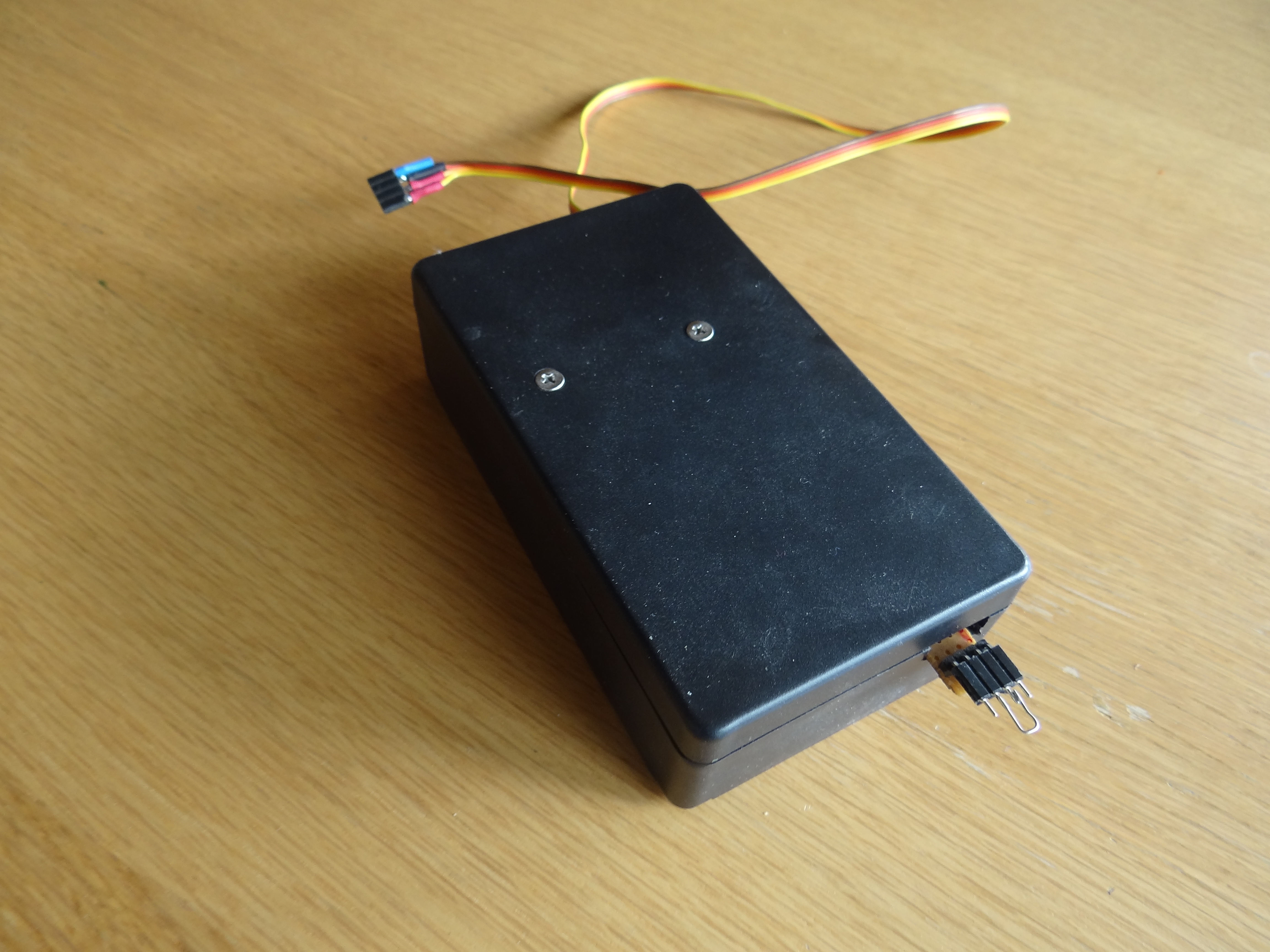
I use it for some of my designs. Others have the batteries
built in, and other are driven by AC power supplies.
News for GPS
The GPS logg was down for some time. Without much hope
I bought a new GPS receiver, of the same type as I
had before. To my surprise that worked. The problem was
that there had been very few position fixes for some
time.
I've built the system into a little round plastic box,
which I can carry in my pocket (it is not the worlds
smallest plastic box, but its OK). Nothing electrical
comes out of the box, and the box is waterproof.
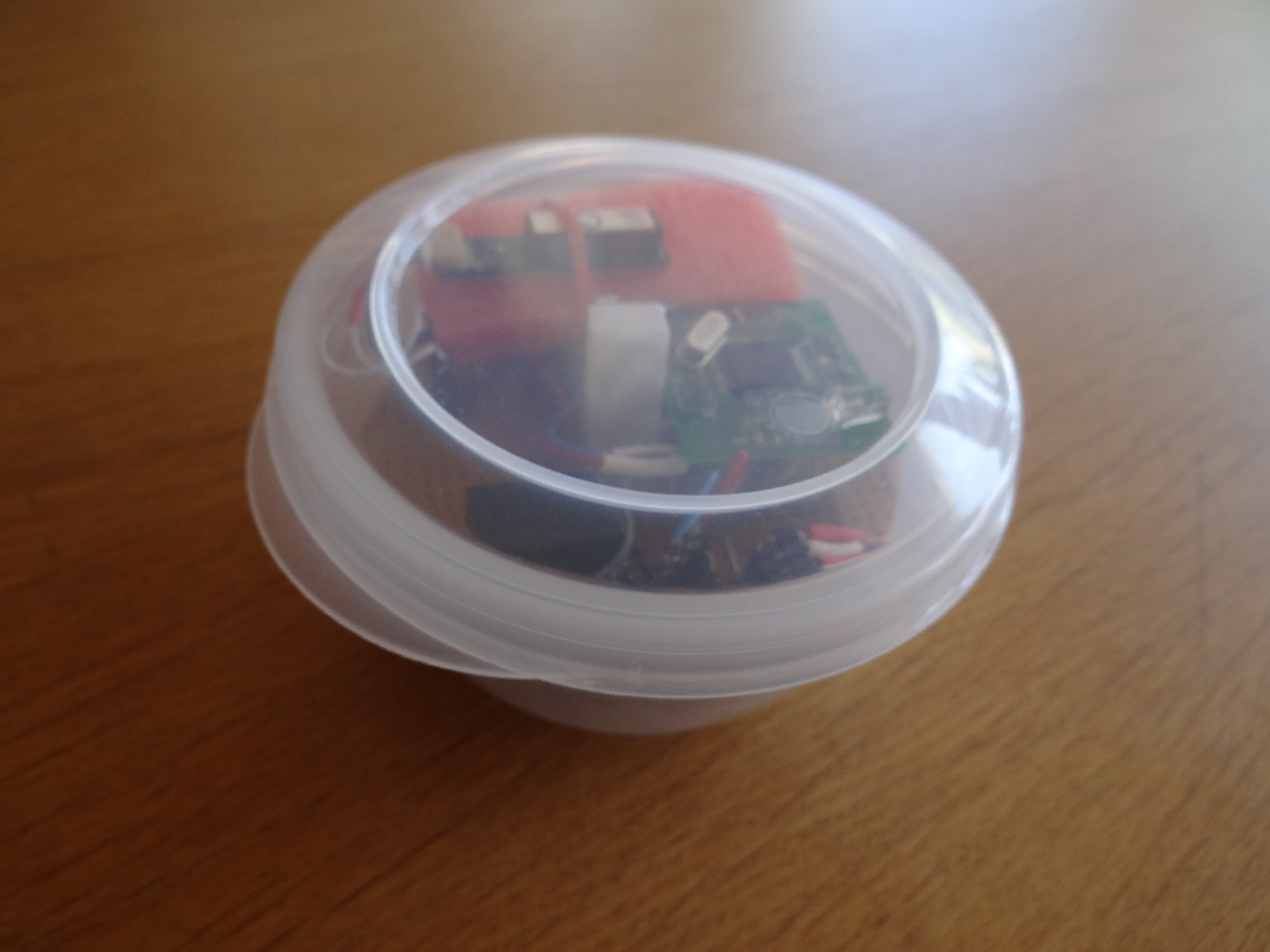
I have also simplified the storage in the on board
memory a little. The new file system for this is in
the file filee2 .mpo. The files are no longer fragmented.
The data are stored in a long array at consecutive
adresses. The current adress for storing is saved
in the EEPROM itself at a given adress (32). The
data array then starts at adress 33. Below 32 is
a "file catalog". The files don't have names; they
just have numbers. The first adress for each file
is stored at that number. Up to the reserve word 32,
there are 31 such slots, which make up for the file
catalog.
The point is this: If there is a power failure,
but the system starts up again, the startup
procedure will create a new file. It gets its
place at the first free slot in the file catalog,
and from there it points to the first place for data,
which is at the adress after the adress stored
at position 32.
We can now see that data have been distributed
over more than one file, and we can paste these files together.
But we can also pretend not to observe this, and just read
all the data as a single long file. It will contain
points of discontinuity, if the power interrupts
have been long, but it may not be harmfull.
Like previously we need a reset program for clearing
the file system. It resets the 31 first positions to 0
and clears the content at adress 32 to 0. In fact, it
clears some more EEPROM words, just to make the
action a little more visible.
More important than these things, is the switching to
Linux, which requires a new procedure:
- Supply the device in the box with power from
the batteries, by installing a little plug.
- Connect the Prop plug, and reset the system by
loading the program gpsreset.mps
- Load the program gpslogg.mps,
or interrupt the power for a short while, so
that gpslogg.mps is reloaded from the Propellers
own EEPROM.
- Close the lid, and go for your adventure, with
the plastic box in your pocket.
- Back home, open the lid again, instert the prop plug
and load gpsread.mps
- Open the screen program in Linux at your
PC. Hit any key, and your data will come flying.
- Press ctrl-a and : and hardcopy -h filename,
where filename is a filename you have just invented.
You should run screen from a directory you
know, so that you can find the files.
- Run the Java program GPSget filename.
This will make a plottable file p[filename].dat.
- Run, optionally, the Java program Dist filename
to get a file p[filename]V.dat, which
also contains velocity and distance information.
- Run the Java program GPXget filename
to get a file, [filename].gpx which you can plot
in a geographic map.
On that last point, Google Earth seems to have abandoned
its services for plotting gpx-files. I found the website
share.mapbbcode.org, which works just as well.
Open the website, and hit the "import" button,
and choose your file filename.gpx, and the system
will zoom in to your track.
Downloads
Most files are unchanged from previously, but
filee2.mpo is new, and the Java files may have changed.
Some of these files have an added '2' to their names, to
distinguish them from earlier versions.
The three Java programs import a package called std.
It is my own standard Java package. You have to create that
package by importing the following three files, which make
a package by mentioning the keyword package std.
Definitions
Many languages allow you to define symbols,
and assign values to them, without reserving space
for any variables in the computer memories. The
symbols are handled by the compiler only.
I found it worthwhile to introduce this in the
MPS language too. Syntactically, the symbols
are single lines defining a symbol name and
its value, like
badluck = 13
Such definitions are placed in .mpo-files
between the keywords defs and enddefs
The definitons are then loaded with a load-command
load from (Termi.mpo)
*defs
i.e. the same way as a function is loaded from an
.mpo-file.
Then the mps-program can use the definition
with the code ?badluck The question-mark,
would mean "What is the value of this symbol?".
The compiler will then replace "?badluck" with
the value 13.
Here we don't need to store the value 13 in a
separate variable in the Propeller.
But the Mps-code is more readable, as
we can figure out what the number is supposed
to mean, or represent. The compiled code
(Propeller assembler code), on the other hand
is not more readable, but it is not supposed to
be.
The Terminals
The Terminal
Here's the terminal:
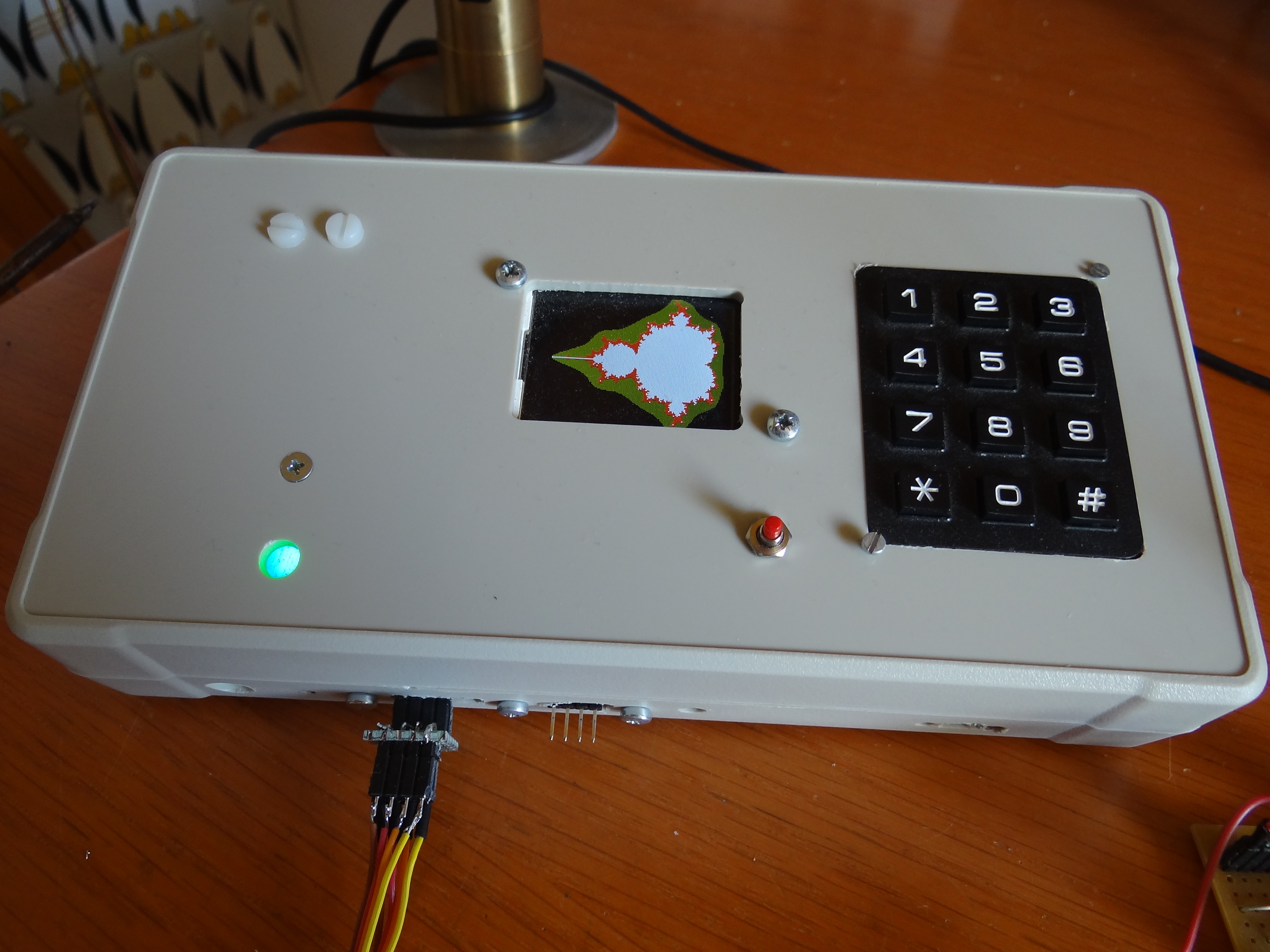
It is a box that contains:
- Some serial RAM memory
- An SD card holder
- A numerical keyboard
- A graphical display
- A three color LED (RGB-LED)
These things are offers of services for a less equiped
Propeller computer (the host). By sending orders
over a link to the
terminal, data can be stored and recovered or typed on
the display, entries from the keyboard can be captured
and the RGB-LED can be made shine.
The picture shows an example, where the
Mandelbrot
set has been drawn again, but now with a host using
the terminal. After that, a program has turned on
the RGB-LED with green light, but the graphical
display still shows the Mandelbrot set. The
camera has dimmed the light of the LED pretty much.
It looks better in real life.
The orders are sent as
Morse messages.
In the image above, you can see the link as "rainbow
cable" entering at the front. It contains power, as
5 volts and ground, and a bidirectional Morse link.
On this link, the host sends orders to the
terminal, and the terminal sends acknowledgments
back to the host. (You can also see how the link is
also a bus - an order bus - which continues to some
other terminal)
The host is supposed, not to send any new order, untill
the acknowledgment has arrived.
Physically, the two Morse wires connect pins 26 and 27 on
the respective Propellers.
The terminal software has
- A reccom process to receive the orders
- An acknowledge process
- A number of task processes,
to perform the desired tasks
An order consists of a command which is given
by a symbol in a definition
in an mpo-file
called TermI.mpo. Optionally, there is an argument
associated with the command. The task processes
split the order into command and argument.
The task processes are essentially loops around a
series of if-statements, which check if an appropriate
command has come. If so, the task is executed,
usually with a call to a function. After that,
the execution goes on to a common point, where
the sending of acknowledgments is administrated.
Normally the acknowledgment is the command itself,
but sometimes, when the host asks for some value,
like the content of a memory cell, that value is
returned instead. Right now,
I let the acknowledgment process administrate
this difference, but there is a global variable
x for the value to be returned.
There is also a simple "internal acknowledgment"
at the common point, in that the order variable
is reset to 0.
The host helps itself with an mpo-file
TermI.mpo ("Terminal interface"). It contains symbol
definitions corresponding to the different commands.
The terminal imports these same definitions, so that
the two systems are coordinated. TermI.mpo further
contains a ti.init function, which establishes
the Morse communication. ti.send0 sends
a command, and ti.send sends a command together
with a single argument.
But TermI.mpo also contains some composite functions.
This is due to the fact that a command
can only have one argument. A typical example is the
task to fill a rectangle on the display with a
color. The terminal will need to know the boundaries
of the rectangle as N(orth), S, E and W -limits, and the color.
These arguments are set by orders like setN, setS,...
and setcolor. A composite function
( N , S , E , W , color , )ti.fillrect
creates these suborders, and also the final order,which
fills the rectangle. This makes the writing of
host software easier.
There is an extra complication with all this.
The reason is that
a single process can't handle everything, that
controls the graphical display. First of all, there
is (as usual) a process for initializing the display.
When its job is done, it leaves over to another
process in the same processor, to do the rest of the
job. But now we need yet another process to handlle
the display.
The display in my case is handled through an SPI
protocol. It means that pins are connected to
pins on the display for clock, MOSI, MISO and enabling.
It is easy to see, that a Propeller has 32 pins (GPIO-pins).
But in fact it has 32 x 8 pins, 32 for each processor.
They are connected to the physical pins through a network,
which essentially or:s the 8 different pins together.
Now if a pin for some processor is 1, then no other
processor can make itself heard; the output is 1 in
every case.
So, what we have to do, is to disconnect a processor's
output pin, when that processor doesn't want to
communicate over that pin. This amounts to changing that
pin into an input pin. For the display, we have a
gra.connect function, which makes output pins.
But now we also need a gra.disconnect function to
make input pins
When the terminal software wants to make something with
the display, it connects to the display. But the other
process has to disconnect itself.
This is handled with an "internal order" in the form
a global variable, called dproc (for "display process")
When a process notices that dproc doesn't point to itself,
it disconnects itself from the display. It also resets
dproc to 0 as an "internal acknowledge". All this is an
extra if-statement in the taskprocess' loop.
The connecting process, say number 1, does its job by
calling a little function as ( 1 )setdproc.
- It stores the argument 1 to dproc.
- It connects to the display.
- It waits 1 ms
The waiting is to allow the other process to
disconnect before the SPI bus is used.
With this, the terminal works exactly as one would wish.
After it has sent its acknoledgment, it is ready to handle
any order. It doesn't need to be turned off, ever. You can
reload the host with new code, and run it directly without
resetting the terminal. (You can see this in the picture,
where one host program has drawn on the display, and another
has turned on the green light. Both these effects persisted,
so that I could photograph them.)
The terminal hardware is displayed here:
At the left is the Propeller's own EEPROM. It needs a
pull up resistor, which is omitted in the figure.
At the far left, you see the input from the host, including
ground and 5v, and the bidirectional bus between the
host and the terminal, which is connected to pins 26 and
27. (There is a diode at one of the wires. I will
comment on that later).
The host delivers 5v which has to be reduced to
3.3v. (I could deliver 3.3v from the host, but I fear
that I could overload the host's 3.3v stabilizer.)
Then, there are 3 SPI-buses for communication with
- the graphical display
- the serial RAM
- the SD-card
The graphical display has the standard SPI-signal
(clk, MOSI, MISO, chip enable) but additionally
a d/c-pin to mark sending of commands/data, and a
reset-pin. At the reset output, there is a little ring
which represents an inversion, done with an external
inverter chip. You might think, you could just as
well do this inversion with software, but the problem
comes, when the Propeller starts, and the program has
not yet started.
The RAM and SD-card share a single SPI-bus with
identical clock and datapins, which is OK, as these
pins are driven by different processes. You can't
use these two buses simultaneously, but the
terminal software never does two things simultaneously.
The RAM consists of four chips, and thus needs
four chip enable wires. The SD-card does with just
one
The keyboard is a network of switches. The figure below
shows one of the 12 switches, the one closed when key "0"
is pressed.
These switches connect one row line and one collum line.
The numbering of these lines is shown in the
figure. The numbering is a little iregular, but it seems
to be an "international de facto standard".
The output from the collums send voltages to the Propeller,
and these inputs require some pull down resistors, as is shown
in the previous figure. In the software downloads,
you can find an algorithm for finding out which
button - if any - has been pressed.
Finally, there is a catchkey process running in
parallell with everything else, and which maintains
a value of the global variable key which is the
current value of any key pressed on the keybord
(if no key is pressed, it delivers 15).
A getkey order will deliver this value as
an acknowledgement to the host.
That same
process also handles the RGB-LED, helped by an object
file col.mpo. It contains two functions:
- (index)colormix
- (on)shine
They are activated through orders colormix
and shine. 'index' is a pointer into a
limited set of standard colors. The LED is controlled
with a PWM system. If the argument on is 0,
then the light should stop shining, but I am not
absolutly sure about that. The shine PWM-system is
run in the shine function, which is called from the
catchkey process.
Orders
The following orders could be found in Termi.mpo as
definitions. I split them into some categories.
Texts within [ ] are comments.
- RAM orders
- raminit
- setchip(chipnr)
- setwadr(adress) [writeadress]
- setradr(adress) [readadress]
- write( data )
- read [read; the value in the acknowledgment]
- Echo
- echo( x ) [x returned in the acknoledgment]
- SD card
- sdinit
- sdconnect
- sdsetwadr(adress)
- sdsetradr(adress)
- sdwrite(data)
- sdread
- sdflush
- Graphical display
- grainit
- cleartext
- appendtext(char)
- flushtext
- setE(coordinate) [set Eastern boundary]
- setN(coordinate) [set Northern boundary]
- setW(coordinate) [set Western boundary]
- setN(coordinate) [set Southern boundary]
- setcolor(color) [16 bits of color information]
- makewin [make window]
- fill [fill rectangle]
- sendhpixel(byte) [send half of pixel color info]
- Keyboard
- RGB-LED
(In this list, I have placed the arguments of
the command after the command, unlike my
convention in MPS.)
sdflush means the following. When writing to the
SD card, you first write to a buffer in the Propeller.
The buffer is written to the card, when it is full.
sdflush means that the buffer is written anyway.
read, write, sdread and sdwrite include that
the adress is incremented.
Text can be written to the display in the following way:
- A cleartext order clears a text in the terminal.
- A number of characters are loaded into that text
whith an appendtext(char) order.
- A flushtext orders draws the text at a fixed
place on the screen.
This is handled with the ( adr )ti.stype composite function
in TermI.mpo. adr is the adress or the text to draw in
the host computer.
Downloads
Termtest.mps is a test or demonstration program.
Look into it and try to guess what it tests.
Term.mps is the terminal software. TermI.mpo
is the
interface between Termtest.mps or any other host program
and Term.mps.
The Analog Terminal
Analog inputs and output might be nice parts of
a terminal. But the terminal box is full, and most
of the Propeller's pins are used. So I made a
new, analog, terminal. It is not so picturesque,
but I will still show a picture of it further down.
Here, instead, a hardware diagram of it.
It has
- An analog to digital converter ADC, MCP3208
- A digital to analog converter DAC, MCP4822
- 3 double power amplifiers to drive motors, or
other such things.
To the upper left, you can see the orderlink to the
host. Here I will explain the
diode in the acknowledgment line back to the host.
We have two terminals now. And both want to send
acknowledgments. The Morse communication "rests"
at zero. Hence, to be able to send messages from
two or more sources, we need to or the
signals together. The diodes are parts of an
"oldfashioned" hardware or-gate. Another
component required is a parallell resistor at
the host's input pin. Without it, the impedance
of the propeller's CMOS input, might very well
exceed the backward impedance of the diodes.
The ADC and DAC are straight forward SPI-components.
The ADC has 8 input channels. You choose them with
the SPI protocol. In the order, the channel choice
comes as an argument. The DAC has two outputs. You
choose the channel with two different commands. Both
take the value to convert as an argument.
There are four "free" analog channels, going to
input pins of the terminal. There is one channel
connected to a potentiometer with a knob at the
panel. Two analog channels are reserved for the
touch screen. All four outputs of the touchscreen
are connected to
Propeller pins, but two of them also go to two
analog channels. They are controlled from functions
in the Touch.mpo object file. How they work is
described here. (In fact,
I thought that the touchscreen was broken. These
Nintendo screens are not easy to find nowadays.
But, I tested it, and it worked!)
The power amplifiers are parts of so called
H-bridges, each with two amplifiers. They come
in pairs in modules. I have two such modules,
so I have a total of 8 such amplifier, but I
have only connected 6 of them. They should
be regarded as "binary", so you feed them with
either 0 or 3.3 volts. (What else could you?
They come from Propeller GPIO-pins!)
They could be used to control motors through
PWM (pulse width modulation). They could also
be used to control stepper motors. This is
done in separate paralell processes, which can
be turned on and off with orders from the host.
The parameters to these processes are set in
a task process. There are three pulse width
fackors called pw1, pw2 and pw3 for three
different motors. And there is an angle set
value xc for the stepper motors. The stepper
motor process has a state x, corresponding
to xc. It is the angle of the motor measured
in units of the motor step size. When x and
xc differ, then the process steps the motor
and increments x, which goes on untill x=xc.
Hence xc is a motor angle command, though
with an undefined null point.
Here now, a list of orders to the Analog Terminal:
Analog input
- adcinit
- adcget(channel) [analog value as ack.]
- touchinit
- touchget [x and y packed together as ack]
Analog output
- pwminit
- pwmx(pw1)
- pwmy(pw2)
- pwmz(pw3)
- stepinit
- steppos(xc)
Just a reminder: If the host wants to send an
order adcget(channel), it makes the following
function call:
( ?adcget , channel , )ti.send
The output from the touchscreen can be called xy.
If it zero, then the touchscreen isn't touched.
Oterwise you can find x and y with:
xy >>8 ->y
xy &355 ->x
Downloads
-
Aterm.mps
-
TermI.mpo
-
adc.mpo
-
DAC.mpo
-
Touch.mpo
-
std.mpo
Here finally, the promised picture of the Analog
Terminal, sitting under the Terminal. They cooperate
on the task of drawing a picture from the touchscreen
on the display.
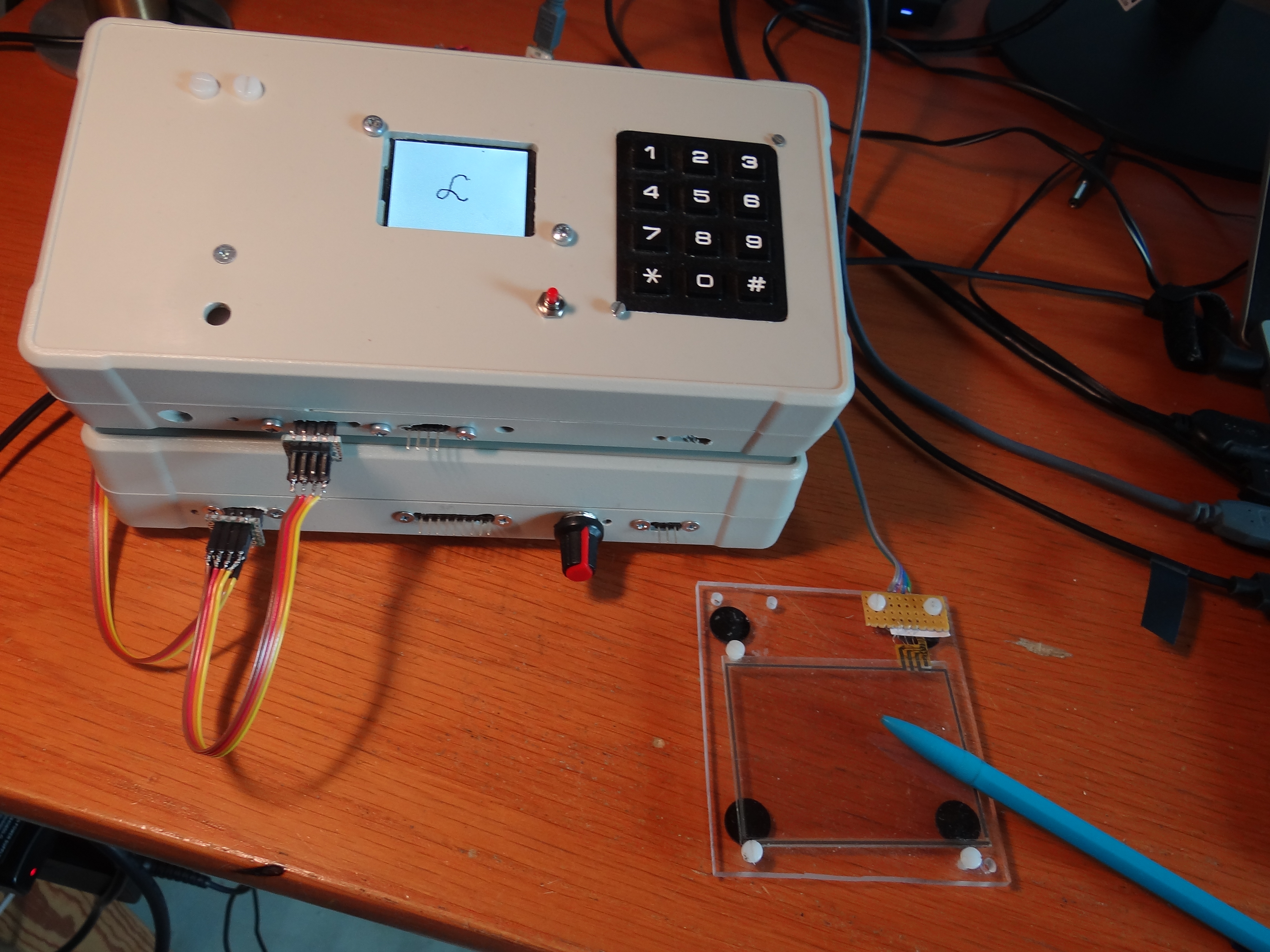
You have seen this
before, but now this is made
as an application
of the Terminal Order System.
(The terminal has a
foot, so that it slants a little outwards, to make
the reading of the display easier.)
The program is called Rita (draw in Swedish),
and can be downloaded
here
The parallel RAM (PRAM)
The serial RAM of the terminal is too slow for some
purposes. Hence I have also built circuits for a
parallel RAM (PRAM). So far, there is not space for this
hardware in the terminal box, but that may change.
From a systems point of view, a PRAM is a simple
component. You give it an adress and a datum, and
activate a write enable signal (WE). Then you can
give the same adress, and activate an output enable
signal (OE), then the datum written, will appear
at the same pins of the memory chip.
The PRAM used is called bs62lv1027 and is from
Brilliance Semiconductors in China or Taiwan. It
contains 1 Mbit in the form of 131000 bytes (128 kBytes). That
requires 17 bits for adressing. To that comes 8
bits of data I/O and one OE and one WE. That
is very much, if we also want a Propeller to something
else. So I decided to add a special memory Propeller.
If we call the other Propeller the host, we
divide the labour between the two like this:
- The memory computer provides the 17 adress pins.
- The host computer provides 8 data lines, and
the OE and WE signals. The data pins connect the
host and the memory to something which is a
bidirectional bus.
- The memory computer gets commands from the host
to set and increment adresses. These orders are
sent through 2 lines connecting the 2 computers.
- The memory computer gets a command to set a
base adress. This is controlled by Morse signalling,
while Morse signalling would otherwise be too slow for the
other tasks.
A host Propeller and the memory Propeller arranged on
two separate cirquit boards are shown here:
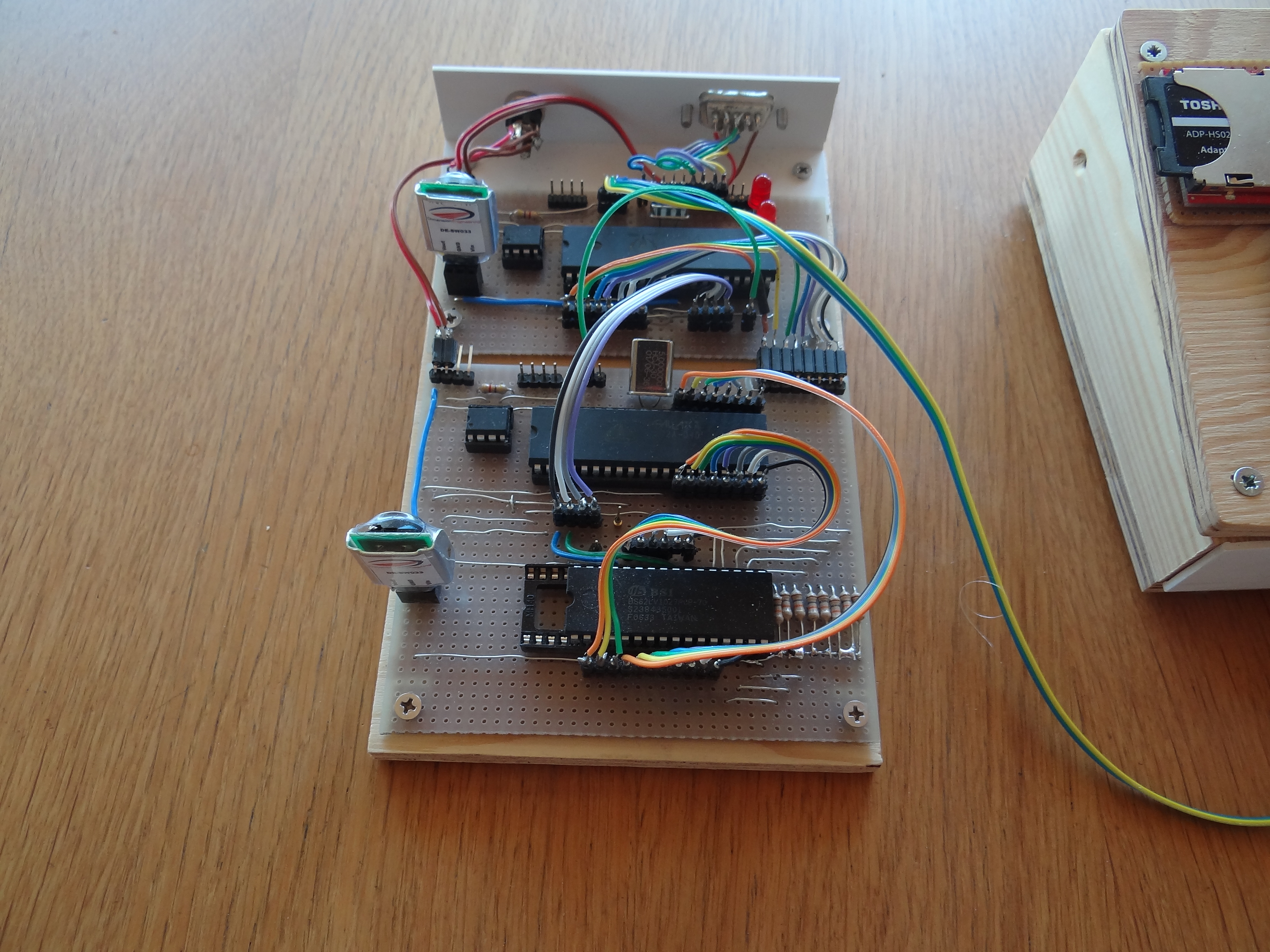
So, now the memory Propeller is just a simple adressing
slave.
Like the object file TermI.mpo, there is a file MemI.mpo,
with functions for handling the PRAM.The Morse code for
setting the base adress, is pushed in in the row of
Morse codes for handling the terminal. I think it would
be possible to build a Morse bus for communication between
host, terminal and memory, but so far, I have separated
the communication lines.
Here are the functions of MemI.mpo
- )memi.init for intialization of the
communication with the memory computer.
- )memi.baseAdress for setting a fixed
adress reference in the memory computer. Sent
with a Morse message with the command code 18.
- )memi.getAdress (currently deprecated.)
- )memi.resetadress for moving the reference
adress to the current memory adress.
- )memi.dirwrite for directing the data
connection from the host computer to the memory.
- )memi.dirread for directing the data
connection from the memory to the host
- )memi.write for writing the memory, i.e.
activating the memory's
WE pin, and then incrementing the adress.
- )memi.read for reading the memory i.e.
activating the memory's
OE pin, and then storing the result in the
host computer, and then incrementing the adress
Downloads
Memtest.mps is a test and demonstration program.
It stores and remembers ascii codes for characters
from '0' and up to '?'. There are some unused processes,
that you can try. runtest types the text
"Eva Skarman" every time you hit a key.
writereadtest is a process that rights
and reads the memory in a single process.
MemI.mpo is an objectfile
for handling the memory from the host. MemA.mps is
the code for the memory Propeller (the "adress slave").
The SPI-camera
Once, I happened to be too generous with supply voltage
to my digital camera C329. So, it went
to its fathers. Then I thought it would be interesting to
buy the SPI-version of it instead of the RS232 version.
This turned out to be quite an adventure.
Getting hold of the camera wasn't so easy, and I haven't
found any competitor. At the same time, the manufacturer
seems to be very anonymous. They have published a users manual
for the RS232 version, and then they publish almost the
same users manual for the SPI version. But the difference
between the two interfaces is important.
In the new manual, they teach us how to change the baud
rate of the camera, while a SPI device doesn't have a
baud rate. The host simply determines the baud rate, as
it provides all the clock pulses. Borrowed from the
RS232 is also a sync command. A sync command is completely
irrelevant for the SPI-protocol. Then, I thought, that
they maybe have a formal requirement on a sync command,
just to start the camera. So I wrote sync command software,
hopefully to delete, when everything works. So, now I have
deleted all that sync stuff!
So now I have an init routine, that sets up the properies
of the camera. And I have a get routine, to ask for
a picture. You find these in the code to download.
Then the picture will come flying over the SPI-line,
but before that comes and acknowledge signal, and a
data signal, telling you about the size of the image
(which you could well calculate youself, based on your
get-order).
But then, and some people on the internet agree on that,
it happens either, that no picture ever comes, or that
not even the acknowledge comes. Everything you clock in
is just zeroes. The recommended trick here, is to try again.
Send the get command again, and see what happens.
4 or 5 tries may be needed. I wonder why that is so.
This retrying is part of the code, so you don't need
to do anything manually.
A problem with the previous camera was, that it was
difficult to see, where the bytes from the actual picture
started. There used to be a heap of extra bytes of unknown
origin. With SPI this was a little easier. If you start
to catch the bytes quickly enough after you sent the
get command, you will see a number of zero bytes. The first
byte received, which is non zero, is usually the first
correct byte from the camera.
Color information from each pixel takes up 16 bits, i.e.
2 bytes. So if you drop one byte, you get out of phase
with the color information, so you get false colors.
That happens sometimes, and the only thing I know to do
about it, is to try again (manually now).
From then on, everything is fairly simple:
- You (i.e. the host computer) sends the init command
to the camera.
- Then you wait for some key, that acts as a shutter
key.
- When the shutter is pressed, the camera gets its
get command
- The bits arrive, and you store them in the
PRAM memory.
- When a display button is pressed, these bytes
are sent to the display of the
terminal with the terminal interface functions
- It is, of course, possible to send that byte stream
to the terminal's SD-card
- However, so far, I have preferred to send the bytes
so the PC, where I can pack the bytes into a file, which
I can store and display.
Downloads
I use the screen program in Linux to get the data.
The principle is the same as for the
new GPS. Then I can draw the picture with the Camera.java
program with the file name as argument. Here's the download:
Camera.java
You need the std.package. Handle that as for the
new GPS
The Universal Instrument
Well, "universal" is a strong word. So what is it?
- A USB oscilloscope.
- A digital instrument for period times,
frequency, capacitance, resistance, voltage and
4 digital inputs.
- A stop watch and an egg clock.
- A pocket oscilloscope.
Here's a picture:
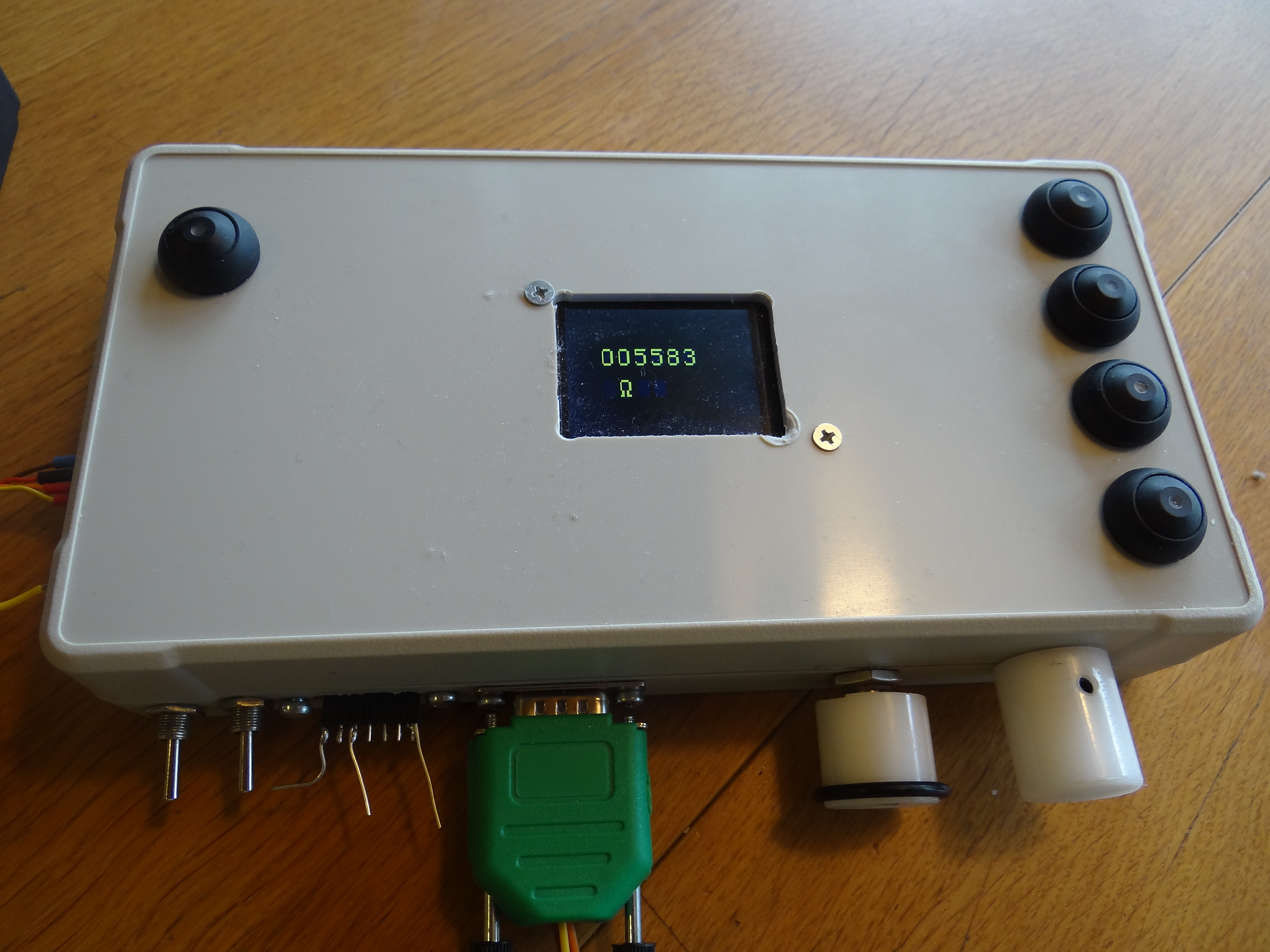
You can just anticipate a black box, which is a power
supply as desribed earlier. It delivers -5,0,3.3 and 5 volts
through a rainbow cable, and a barely visible connector
on the left side. The power source in the box is
two Litium batteries. Most signals come in through the
Dsub9 connector. The knob next to the right is an
analog potentiometer, which chooses modes for the
instrument. The buttons on the right side of the
panel, are used for control of the programs. We call
them b1 (at the bottom), b2, b3 and b4. The
button top left on the panel is for reset of the
software. The display shows the resistance of
5.6kΩ resistance built in to the system. There is
also a 2.2μF capacitor. You can disconnect these
components with the switches to the left, so that you
can measure external "unknown" components. They are to be
connected to pins beween the switches and the Dsub
connector.
A simple MPS program can't contain all that, so the box
has four EEPROMs, each with its own program for the different
services. Choose service with the knob to the right, with
values 0..3. After having moved the knob, press the reset
button to the left on the panel. Then a program is loaded
from one the four EEPROMs
Here then an account for the four different pieces
of software in the EEPROMs.
The USB oscilloscope
This is a simpler version of the USB oscilloscope I have
presented earlier. It has two analog channels, with
some analog preprocessing. It is not as ambitious as
the earlier system. Basically it is just two voltage
followers to raise the impedance of the Analog to
Digital Converters (ADC). The ADC:s are simpler than
the ones presented before. They have a lower sampling
frequency, and are controlled by SPI.
Also, If you are more ambitious,
you should have two rotary switches with resistive
voltage dividers, to provide different ranges.
Furthermore, there are four purely digital inputs.
The bit pattern can be displayed either as four
individual bits, och as a hexadecimal number.
These connections go directly into the Propeller
input pins, but maybe you should have some protective
circuits. The Propeller inputs don't tolerate much
overvoltage.
You control the function from the PC. First, open the
Linux screen program. The instrument should be up
and running the USB oscilloscope software (knob position 0).
Hit a key, and your data will come flying.
There are 5 different sampling rates:
~1μs, 10μs, 100μs, 1ms and 10ms.
The first of these is the fastest possible, and it is
pretty close to 1μs but not exactly. But the system measures
times, so the plotting becomes very exact anyway.
The system samples 7000 samples, so 10ms gives you
70 seconds of measurements.
There are 5 modes.
- sim, codes: 0,1,2,3,4
- digital, codes: @,A,B,C,D
- bits, codes: P,Q,R,S,T
- analog codes: ',a,b,c,d
- dual analog codes: p,q,r,s,t
The different codes are for the different sampling rates.
The sim mode is just for debugging. Modify it yourself if
you have some special problems.
The digital mode presents (in the PC) the four
bit bitpattern as a hexadecimal number, while the
bits mode present the
individual bits in separated curves.
Analog is the analog input 1 in that d-sub connector,
The d-sub connector also supply 3.3v to feed an external
cirquit on which you make measurements.
Dual analog logs two variables, and presents them as
separate curves.
When you are ready to logg something, start the Linux
screen program on your pc and
hit the appropriate one of the keys given in the
mode table above. Then data are logged, and then
data are rolling in on the screen window. First comes time
information, so that the time scale on the plots can be
established. Then come all the data. On the screen they appear
as hexadecimal numbers, two per byte, but the figures over
9 are encoded with :;<=>? rather than ABCDEF.
Now type ctrl-a : hardcopy -h hex.dat.
Then run Osc.java without argument, and you get the
plot. A little of how the plotting works can be found
here.
Here's the analog cirquitry, based mainly of an OP290
operational amplifier (two ampliers in a chip).
It's a follower cirquit with 15kΩ resistance. 0Ω could
maybe do as well, but perhaps the 15kΩ resistance
enhances stability. The input resistance of 2MΩ is
necessary. Without it, the input floats around freely,
probably because the ADC pumps out some current. The
100kΩ resistor reduces gain a little, so that the
range +-5 volts can be contained. I have also marked out
the protection resistor between the ADC and the Propeller.
Without it, and driving the ADC with 5 volts, the
Propeller input could be destroyed.
The Digital Instrument
The digital instrument measures voltages, and that is
done exactly with analog cirquitry presented above.
But it also measures resistances and capacitances.
This is done with an RC oscillator. To build such an
oscillator is quite easy:
You use a gate with hysteresis. SN74HC14 is a high
speed CMOS gate, which is very fast, so you can get
high frequencies. The symbol for the cirquit used in
the picture, tells you what hysteresis is. The state of
the system circles around in a rectangle. The frequeny is
proportional to 1/RC.
But the hysteresis levels for these CMOS gates are
a little bit unstable, so I decided to use an analog
comparator cirquit, LM311, instead. It is fast enough,
unless we try to measure small capacitors. These
should generate high frequencie, and the LM311 doesn't
quite manage that, so it might be an SN74HC14 instead,
if that is interesting.
Comparators "traditionally" have an open collector
output, so I need a pull-up resistor, here of 1kΩ.
The three resistors of 39kΩ and 22kΩ, make up for a
positive feedback network, resulting in a very well defined
hysteresis range. Then R and C again define the
oscillation frequency proportional to 1/RC
Now, we have a built in R and C, so we get a fixed
period time and a fixed frequency, which we can measure, as
the output of the oscillator goes into our Propeller.
Then we can disconnect R, and plug in a measurment
object. But we maintain our reference C, and then we
can compute R. And we can do the same, to measure
a capacitor. Furthermore, if we remove these reference
components, and inject a signal into the cirquit, we
can measure the frequency and period time of that
signal (provided it is periodic of course).
We switch mode with the left of the two knobs, and then
we can
see the result on the display. The units displayed
should tell us which mode we are in.
The program tries to scale the results, and select
units, so that it shall be easy to understand the
result.
The Stop Watch and the Egg Clock
This program is really quite simple. You can improve it
a lot, e.g. introduce minutes (now everything is just
in seconds). It has two modes, and they are selected by the
left knob. Turned to the left, it invokes the stop
watch, to the right the egg clock. Now remember that the
buttons to the rigth, from down an up are called
b1, b2, b3 and b4.
In stop watch mode, b1 starts the timing, b2 stops and
b3 resets time to zero. You see the time on the display
in cs = s/100.
In egg clock mode you move a starting time up with b1.
If you go too far, you can move it down with b2.
b3 starts the countdown. When time passes zero, a buzzer
beeps for 1 second.
The Pocket Oscilloscope
Well,... you need to have big pockets! But you can
miniaturize the thing if you want. On the other hand, the
idea would be that a battery driven little instrument
could be easier to carry around than a PC or a standard
oscilloscope. But, the display is small and has a low
resolution, and I haven't put any work into writing
numerical data to the display; you just see a curve.
You start the logging with button b1, and then data
are logged in the Propeller's global memory (same as for
the USB oscilloscope). Then the display is erased, which
takes most of time used, and then a curve evolves.
As the display resolution is
low compared to the 7000 points we logg, most signals will
be heavily undersampled. But then we can expand the figure
with a factor of 2, for every hit we make on b3.
We can compress the picture again with button b4.
While we do these expansions and compressions, we see all
the versions of the picture at the same time. This looks
a little messy, but we have some chance to see what
happens. When we want to see the picture clearly, we
hit b2 to erase the screen, and then the latest version
of the curve will appear.
This overdrawing is helpfull, as we don't have to wait
for erasing beween all the pushes on b3 and b4.
In this picture, you can see a logging of the
instrument's RC oscillator signal. The image is expanded
a couple of times. The period of that signal is slightly
less than 1ms. There is no choice of voltage range;
it is fixed to 0..5 volts.
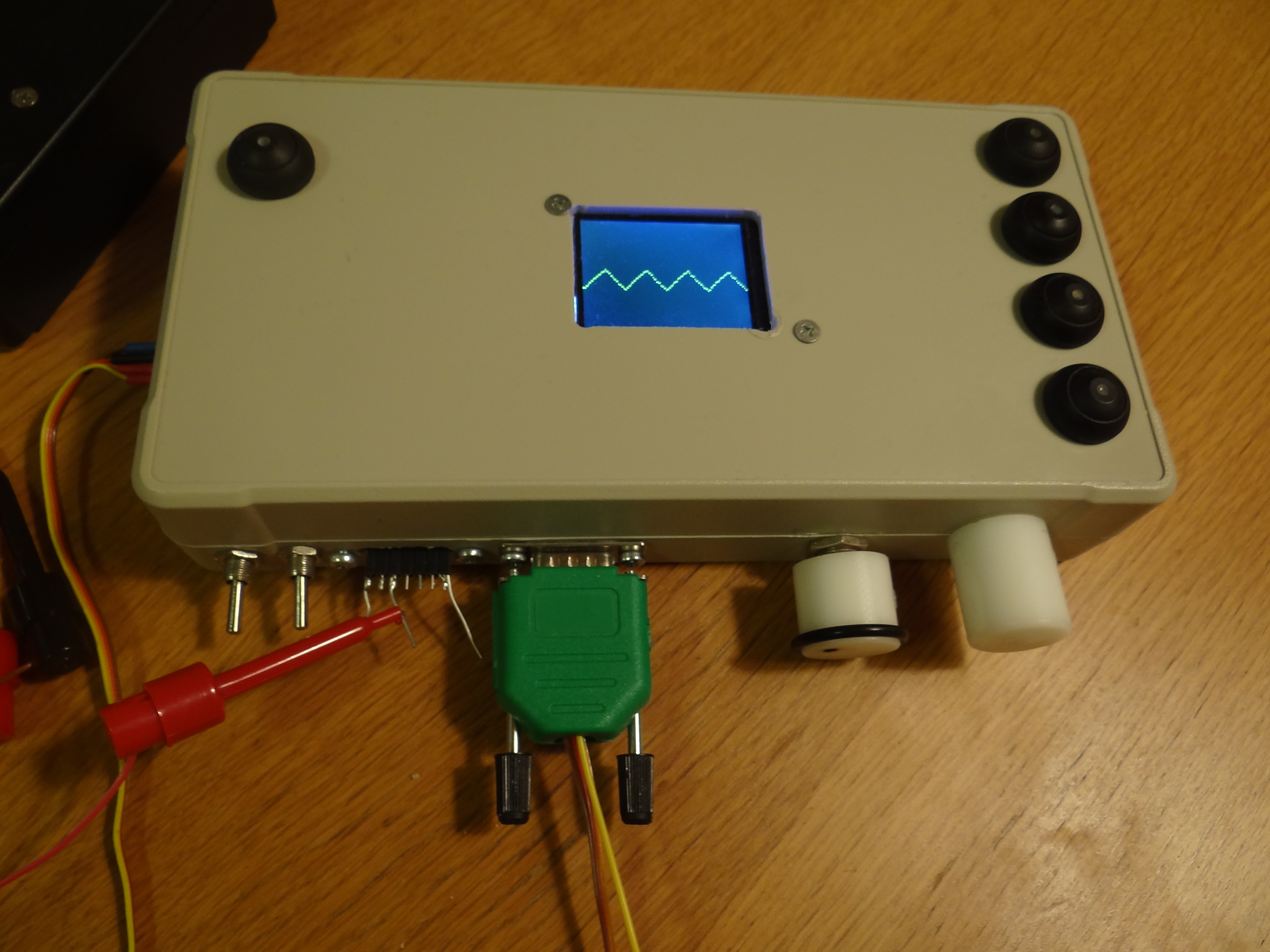
Downloads
A USB oscilloscope
I found it handy to build the USB oscilloscope into
a separate box:
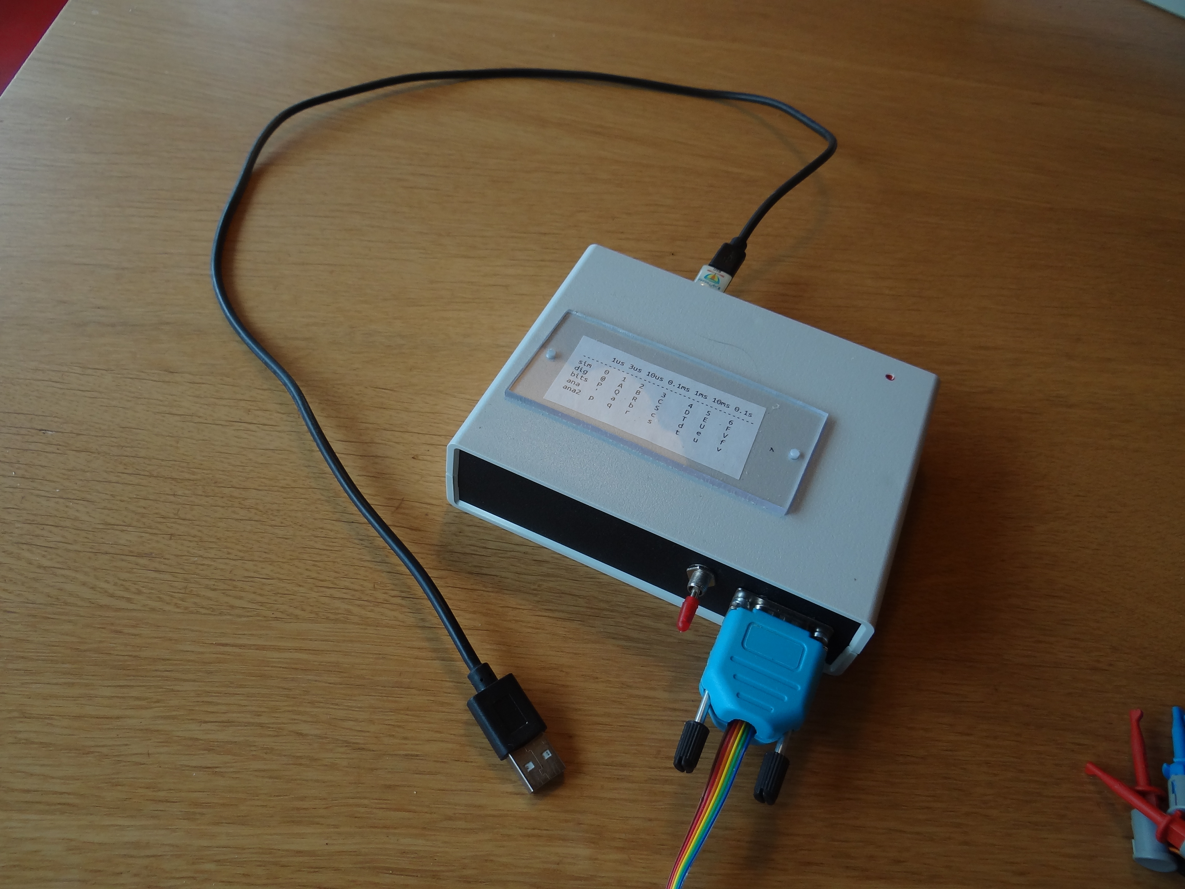
It has two chargeble Litium batteries, and a little
label, that gives the codes for the different modes
and sampling rates. On the back it has a connection for
charging the batteries, and the connection for a
propstick for the PC communication.
Connect your signals to the D-sub connector, your
PC to the propstick, open a Screen window on the
PC, hit the appropriate key on your PC, and see you
data come flying. Save your data with this command
in your Screen window:
CtrlA : hardcopy -h hex.dat
Then call the program Osc.java, which reads data from
that file hex.dat, and displays the result. It allows
you to zoom into the plot.
Here's an example:
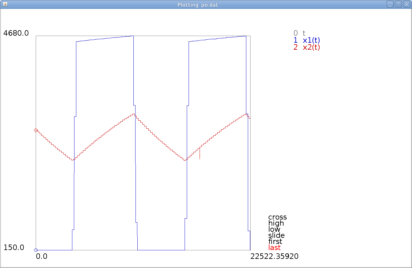
This is an analog plot with two signals. They come from
the RC oscillator in the Universal Instrument. So it's
a square wave and a sawtooth wave. You can se a sampling
effect where you get staircases where the squarwave jumps
up and down, and you can see some disturbances, like the
spike in the sawtooth. At the top of the square wave you
can see that the line is slanting. That's because the
comparator has open collector output, so you put a resistor
up there, and it gives a "non zero time constant". The
accuracy in voltage (given in mV) is as good as my
calibration of it. The accuracy in time (which is given
in μs) is as good as
the Propellers crystal, i.e. very good. The frequency of
the signal is 85 Hz, which can be measured from the plot with
great accuracy.
You can recognize that triangular wave from the
"pocket oscilloscope".
Here a digital example, which may be even more interesting.
A USB oscilloscope is actually very effective for
analyzing digital communication. We try to use the
I2C protocol to communicate
with a camera called OV7670. It didn't work, partly
because I never connected that camera, but in fact
I've never seen a sign of life from it. But we can
at least see the host computers efforts with the
communication.
We have a plot, and now we have zoomed into the plot
to see the beginning of a conversation:
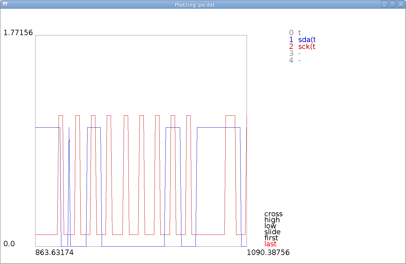
The red curve is the clock signal (sck). The blue curve
is the serial data line (sda). First we see how the
blue line falls while the red line is high. That
should maybe be forbidden, but it is interpreted as
a start pattern. Then comes a blue curve spike.
Maybe it shouldn't be there, but it comes when there
is no clockpulse on, so it is harmless.
It is followed by the bit
pattern for hexadecimal $42, which is the official
I2C adress for this type of camera.
Then the slightly longer clockpulse is for clocking in
an acknowledge signal from the camera. It should be
a zero on the blue line, but it never comes.
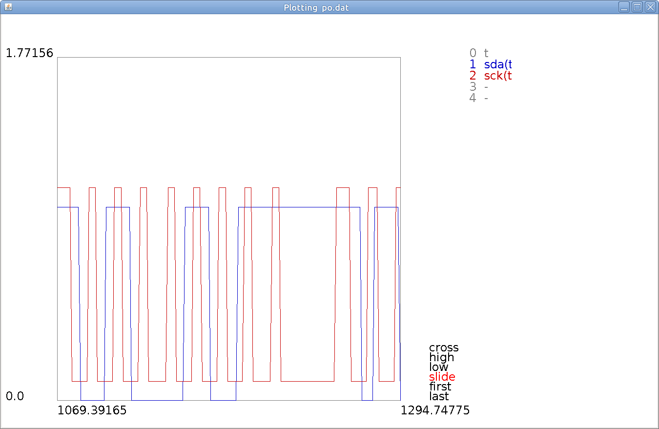
The camera has a bundle of registers, that we want
to read. So we send the number of such a register, which
happens to be $4B. Again an acknowledge clock pulse,
and still no acknowledge signal. Finally we see a
stop signal followed by a start signal (blue lines
moving up and down during the duration of the clock
pulses.
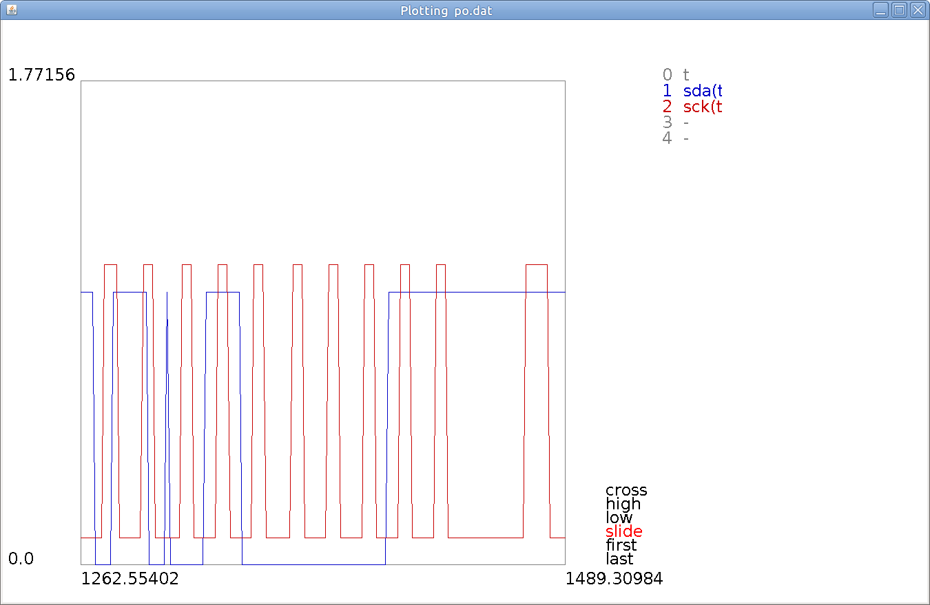
(Firstly, the stop and start patterns seen in the previous
plot, appears again).
Now adresses have been sent, and we want the camera to
know, that we want to read from it. So we send
the $42 again but now augmented with a readbit 1,
so we send $43,
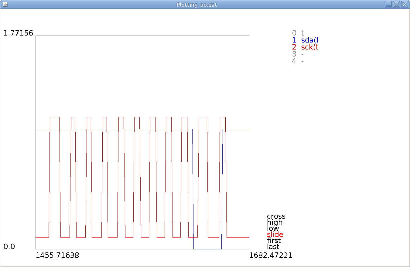
The result then is 8 bits being 1, which makes up
for the hexadecimal number $FF. But then
(miraculously?) we get an acknowledgment 0. But
this is no miracle. This is an acknowledgment that
the host should send, in thankfullness for the
data it got. And it did send that acknowledgment!
The Automatic Trumpeteer
In December 1813 Ludwig van Beethoven organized
a concert, not with his own music, but with a
"Jubileumskonzert" by Ignaz Joseph Pleyel. It was
a chamber orchestra accompanying an Automatic
Trumpeteer, designed and built by Johann Nepomuk Mälzel.
The trumpeteer was a wooden doll playing a real
trumpet hardware. Trumpets at that time, had no
valves, so they could only be played with so called
"natural tones". Those tones were generated with a
vibrating reed placed in the airflow into the trumpet.
The programming was made in a mechanical arrangement,
somewhat like a punched card.
The concert was reperformed lately, now with the
programming made in a microprocessor.
My automatic trumpeteer is even simpler:
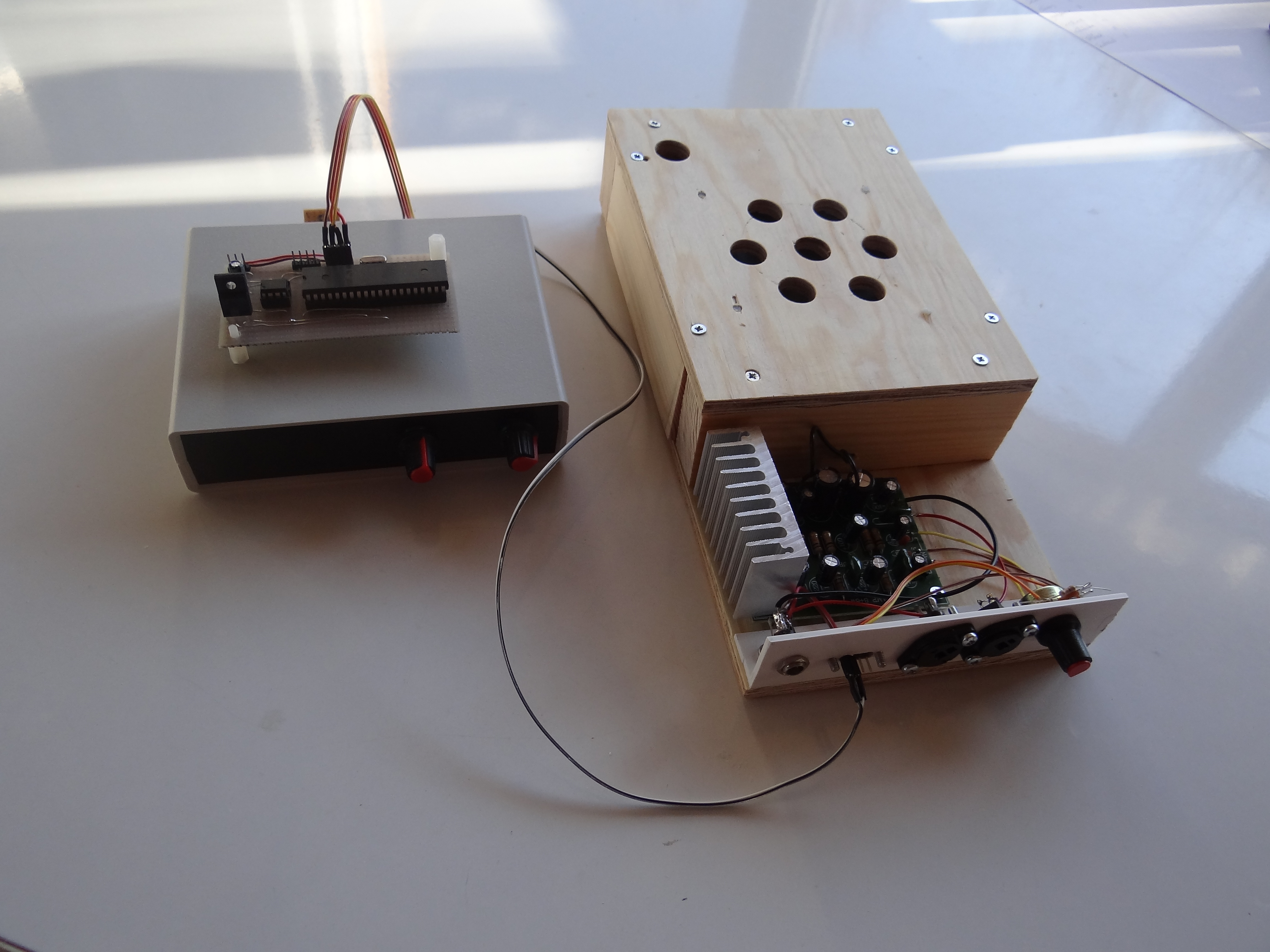
To the right, there is a loudspeaker and a power
amplifier, which is a kit from Thailand. The box
is a computer controlled tone generator, which
generates sine or trianglewave outputs (sine waves
are a little dull to listen to) with very accurate
frequencies. Volume is also controlled, and the
tones are also damped out with a chosen time constant.
So, then, this is maybe rather an automatic piano.
The "piggy back" on the box, is the machine, that
produces the commands to the tone generator.
These commands are controlled from a file, which
describes the music in terms of musical tones.
I use the standard names of tones like C,D..A,H
followed by an octave designation. A white space
is for the standard octave containing A = 440Hz.
A - is for the lower octave, and ' is for the higher.
Then follows a white space or a 'b' for lowering the
tone. So this is a piano. We dont distinghish between
G# and Ab. The scale is the welltempered scale made
famous by Bach in his "Das Wohltemperierte Klavier",
but probably invented by Simon Stevin. It has 12
tones over an octave separated with a factor of
the 12th root of 2. Then, the length of a tone is
given in 1/32 fractions of a full note.
These notes are given on a file *.mus, which is
transformed into a more numerical file *.myd.
I have some file systems, like those based on
SDH-cards, but right now, I just import these
data using the global data concept. It means that
the music I play, is compiled into the
code.
The music computer sends frequency and volume
commands as Morse codes to the tone generator.
The Morse code for frequency gives the frequencies
in Hz. The decay of the tones is made by the
tone generator with a time constant received in
a "damp" command from the music computer.
The physical length of a full tone is controlled by
the music computer by the pace in which it sends
the commands.
The tone generator first makes a ramp that goes
from the smallest 32bit value to the biggest.
You get such a ramp by adding 429500 to a variable
every 100μs. That gives a ramp of 1s. Then you
can get higher frequencies by multiplying
429500 with your desired frequency. The 100μs period
is made with a wait instruction, but the waittime is
adjusted for the overhead involved in the loop.
Then this ramp is sent through a sine routine which
is based on a sine table in the ROM of the Propeller.
The triangular wave is made by sending the
ramp through an absolute value instruction.
Then, these signals have to be moved to swing around
0 before the amplitude modulation, and then
moved up again to hit the middle of the conversion
range of the Digital to Analog Converter, I'm using.
It's an SPI based DAC, with maybe a little to low
sampling frequency. Higher tones get a little
undersampled.
I'm sorry for having been too lazy to provide you
with a sound file. I didn't have access to
Ignaz Joseph Pleyel's Jubileums concert, so
instead I play a theme, "Polowetsian dance" from the
opera "Furst Igor" by Alexandr Borodin.
Machines like these seem to lack a talent to play
music in an enjoyable way. The same holds for
Mälzels automatic trumpeteer.
Downloads