Propeller Application
Erik Skarman
The Propeller microprocessor
The Propeller microprocessor is a computer developed
and produced by Parallax Inc. It is a 32 bit computer
running at 80 MHz. Its most important feature is that
it has eight individual processors, called cogs,
which operate in parallell. When all these processors
are working, the total capacity of the machine is thus
640 MHz.
More importantly, however, the eight parallell processors
allow you to work easily and nicely with real time
systems, controlling and interacting with "real things".
You can avoid the interrupt concept, with all its
pedagogical difficulties and pitfalls. Instead,
you assign a dedicated processor to monitor events from,
say, a sensor. When it detects the event it can grab
some external signals and then invoke computations in the
other processors in a very versatile and transparent
way. For the monitoring there are instructions that
monitor an event in a single instrucion, so that the
computer stays within the instruction until the event
happens.
The processors communicate with each other over a global
memory. This memory is connected to the processors in a
round robin fashion, thus avoiding the risk that two
processors try to access the memory simultaneously.
To allow constistent transfers of data chunks with more
than one word, there is a semaphore concept.
The processors communicate with the external world over
32 I/O pins which are programmable to be either input or
output pins. There is a simple scheme for resolving
conflicts between several processors accessing the same
output pins. All input pins are simultaneousy available
to all processors.
The processor also has a real time counter, running through
all the values of a 32 bit word in a few minutes (after which
it overflows and restarts), and
wait instructions that halt the processor (cog) until
the time counter has reached a specified value. In this
way it is possible to contruct very accurate real time
functions.
Content
Programming languages
Propeller Assembler
The Assembler language of the processer is
available to the user through the Propeller Programming
Environment (even though in some sense it has to be
encapsulated in a Spin program). Here is a sequnce of
four instructions which can illuminate some special features
of this assembler language:
sub x,y nr,wz
if_eq mov x,y
if_eq jmp #zero
if_neq jmp #nonzero
Here we subtract the variable y from the variable x,
The result would be stored back in x, but not in
this case, due to the nr flag (no result). Instead
the wz flag commands an update to a z-register. This
z register becomes true if the result was exactly
0 and false otherwise.
The next two instructions are gated with this. They are executed
only if the z-register is true. First we move the value
of y to x (which is kind of meaningless, because in this
situation, x and y are already equal). Then we jump
to an instruction labeled with "zero".
If the z-register were false, the two first instructions would
be executed as no-operation-instructions (nops), and then
the program would execute a jump to the instruction labeled
with "nonzero".
The z-register has a sister, the c-register, which indicates
whether the MSB of the result is 1, but it can also
detect overflow.
This gating of instructions with conditions allows
the building of "if-then-else" constructs without
using jumps.
Spin
The Propeller computer is supplied with another
language at a higher level, the Spin language.
It is an interpretive language. This means that the
programmer is not running his own code. He runs an
interpreter, resident in the propeller, which interprets
the Spin code (somehow encoded into 1:s and 0:s).
This interpretive principle facilitates the design of
a nice high level language. But the whole method is slow.
Given a high level Spin language and a fast Assembler language,
the natural approach would be to write time critical
functions in assembler, and connect them through a Spin
program. To my understanding, this is not the way Spin
and assembler code work together. The Spin "call" to
Assembler code amounts to that a cog is started to run
from the machine adress of the indicated assembler code.
But there is no return instruction to return to the Spin
code.
MYRA
An interest I had in stack programming several years ago,
led me to try to design a stack based higher level
language, that could be compiled into assembler. I was
also inspired to this by someone, who had made a FORTH
programming language system for the Propeller. FORTH
is a stack based programming language, and so is my
language, called MYRA. A documentation of this
language is found here.
But here are some introductory comments.
Stack based programming means that one has a stack
to which one piles up data,and from which one fetches data.
These data are all 32 bit words, and there is no typing of
data. There are producers which pile (or push, as the term is)
data on the top of the stack, and there are consumers who take
(or pop, as the term is) data from the stack.
But they may only take data from the top of the stack.
Thus, when a consumer has consumed one item from
the stack, the item under it is reachable for the next
consumer. Most things in a computer program are functions,
and functions are both consumers and procucers. They
consume the argument for the function, compute the
result and produce the result on the stack. This
interface works for both standard operations like + and
for functions written by yourself. The latter can be
functions written in MYRA, and functions written in
assembler. The functions written in MYRA can be written
inside the main program code, or they can be localized
to external, so called, object files. Assembler routines
are written into an assembler resource file, and at
compilation these functions are put into the compiled
code as needed. This "universal interface" to functions
seems to me to be most important advantage of stack
based programming.
The intended meaning of object files, is that they
should contain functions useful to interface with some
object, like a display, a sensor etc.. If you have
an object file for a display with functions for handling
the display, you can effectively hide the details of
display handling in the main program. To make this
transparent, you should also name functions in object
files with object "dot" notation, disp.write.
A function that most objects would contain would be
an initialization function obj.init. When you call it,
the call can look as follow:
pin [obj.init]
"pin" is the number of the pin, to which you have connected
your physical device. In this way, you can have a single
object file, and use it for several main programs, which
may run in different propeller computers with different
connection configurations to external hardware.
If - then - else statements in myra are written in a way
that mimics what happens in the assembler code. Here's
the example given in assembler above, but now in Myra:
x y - ?
={y ->x >zero}
#{>nonzero}
The important "?"-instruction here loads the status
of the data on the top of the stack to two status registers,
one of which is the z-register. The instructions in curly
brackets are
then gated with conditions. The condition "=" means that
the z-register should be true. The condition "#" requires
the z-register to be false. The instructions in this case
are storing of y into x (storing is represented with an
"->" arrow) and jumps to the label zero and nonzero respectively.
(Jumps are represented with a ">"-arrow)
This way of constructing conditional statements fits directly
to the structure of the Propeller hardware, and it is quite
elegant, but it has its pitfalls. The critical thing is
that code within a curly bracket may change the status
register. This can easily happen if functions or assembler
functions are called. In some cases one should be conservative
and use jumps in the curly brackets. But there are also
instructions to enhance safety. The ! instruction
restores the registers to the value they had directly
after the call of a ?s (set status and save).
There are also instructions S and R to
save and restore this saved value. Read more about this
in the language
documentation .
In the good old Algol programming language, you could have
if constructs inside assignments:
x := if n=0 then 1 else n*(n+1)
That habit seems to have died out after Algol, but here
you can do it again:
n ?
={1}
#{n n 1 + *}
->x
The applications and object files, that I will present
here, will be written in Myra, so that is why, it may
be interesting to learn the language. The files presented
should also be a very good study material in that learning
process.
The Myra System
Here is the software you have to download in order to
use the Myra language:
- Myra.java.
This is the
compiler for Myra. Download this and the other
java files, and then compile using the javac Java
compiler. Run as
java Myra myraprogram
where the filename extention '.myr' is left out.
The compiler will produce a number of spin code
files. The first of them will be called myraprogram0.spin,
and it contains the program for cog 0, which will then
load the other cogs. Normally the other files are
called myraprogramM0.spin, where M is the number of
the cog. If several programs will be run in one
cog in series, there will be names like myraprogramM1,
myraprogramM2 etc. The compiler has a boolean called
machineCode. If this is set to true, Myra will
generate machine code, for the cogs from 1 and up,
though this machine code will be disguised as
assembler code in the form of variable declarations.
In this case, the Myra compiler will print the
number of memory cells used in each cog. If any of
these numbers exceeds 496, the loading of the program
will fail. Open the Propeller environment or the
Propellent environment with the file myraprogram0.spin.
From there, the code can be loaded into the Propeller.
-
Propasm.java. This is an
assembler, which creates machine code from
assembler code. It is only used when Myra.java
has its machineCode boolean set to true,
but it is needed to make Myra.java compilable in any
case. It assembles code from the file Program.asm
to the file Program.bin. It is not a complete assembler.
It only handles the assembler operations that the
Myra system generates.
- Disasm.java.
This is a
disassembler from machine code to assembler code.
It is not a part of the system, but I made it to
help debug Propasm.java.
- codes.txt
contains binary instruction
codes for the assembler instructions. You can augment it
with missing instructions, to help Propasm handle
more programs, but note that some instructions
are distinguished by bits outside the instruction
code proper.
- conds.txt
contains binary
codes for the different conditions if_a, if_nz etc.
- InFile.java
encapsulates
java's file concept to create an input file.
- OutFile.java
creates a java output file.
- Text.java
contains
stringoperations acting on an object Text which
encapsulates java's String concept.
-
StringOp.java. This
is an older system for string operations, that is
used in the older programs InFile and Outfile.
- Assembler.spin.
This is the assembler resource file, which contains
a diversity of usefull (and in some cases indispensible)
assembler routines. Your are welcome to add new
assembler routines to this file, once you have learnt
how to do it.
- Macros.myo.
This is a small file that contains some macros, that can
be substituted into the Myra code.
- Patterns.myo.
This is as yet an insignificant little file, that
contains (so far) one software pattern; a
system for iterating through the elements of
an array. It is used by the file display.myo.
(Sorry for that some of java files are commented in
Swedish. I don't think yo need the comments, but if you know
Swedish, they may be of some help.)
Myra.java starts with
a comment block, which describes the hierarchy of methods.
In the right collum, there are designators for the methods,
and these will reappear at each method, so you can find
the methods by searching for these designators.
The MPS language
I developed the MPS language for the Propeller recently,
in order to get faster code. Historically, however, MPS
is several years older than Myra. In the early 1970:s
I wanted to build my own computer. At that time, one could
buy a chip from Intel called 4004. It was a 4 bit machine.
To add two 16 bit numbers required a full page of programming
code. So I decided to build the computer myself from
loose integrated circuits (counters, adders, shift registers
etc.) The computer got the name Computer 108, as the
computer in the Swedish fighter aircraft Viggen (JA37) was called
computer 107. For it I developed the MPS language, which
was short for My Programming Language in Swedish.
Now, some 40 years later, I have adapted almost the same
language for the Propeller computer. Myra worked on a
computer model with a stack, but the Propeller doesn't have
a stack, so the stack has to be simulated, which is costly
for execution speed and program size. Computer 108 just
has a single register, accu, in which the result is
accumulated. Then most instructions refer to
- a cell in memory (local or global).
- the accumulator register accu.
In the Propeller, the accumulator has to be represented
as a memory cell. Now we constrain our use of the
Propeller instructions, so that one of the operands in
the instruction is always the accu register. This underuses the
Propeller, but it makes it a lot easier to write programs.
Overall structure
The general structure of MPS is the same as for Myra.
There is a system line, declarations of global variables,
an exec lines, which describes how processes are
executed (in parallell and in series), and then a
number of processes, starting with the "process" keyword,
and ending with a "\". In the process, functions can
be called. Functions can be allocated in object files,
now with the filename ending with ".mpo".
A difference is that the MPS system doesn't have any
assembler resource file. As MPS code comes very close
to assembler code in effectivitiy, there is virtually
no assembler code in MPS, but everything is written in MPS.
The functionality of the assembler resource file, is put
in the object file std.mpo.This object file
is used as any other object file.
There is a possibility to write "in line assembler code"
in MPS, but this is used very sparesly, and is incapsulated
in functions in object files.
With this mentioned, the differences between MPS and Myra
code, appear in executable parts of processes and
functions (what comes after the 'begin' keyword).
Instructions
In the executable parts of the program, instructions
are separated with blank spaces and with line feeds
if one wishes to structure the code on several lines.
Binary instructions
The dominating instruction type is the binary instruction,
which has the value of accu as the one operand, and
where the other operand is:
- The value of a memory cell, local or global.
The memory cell i symbolized with a variable name.
This name has to be declared elsewhere. If the
variable name is found among the global variable
declarations, it is a global variable, otherwise
it is a local variable.
- The adress of the variable. In this case,
the variable name is preceded with a '#'-symbol.
- A number literal, if the operand can be interpreted
as a number.
- A character literal, if the operand is a single
character, surrounded by quotations marks (")
- The first cell of the cog memory, if the operand
is exactly "L0". (The meaning of this will be
explained in a while.)
The binary instructions are the following:
- op (the operation itself is "anonymous")
The instruction loads the operand into accu.
- +op adds accu and the operand and places the
sum in accu
- -op subtracts the operand from accu
and puts the result in accu
- *op multiplies the operand and accu
and puts the product in accu. This is actually
a call to the mult function in std.mpo,
which has to be mentioned in a load statement.
- &op makes a bitwise and between accu
and the operand.
- |op makes a bitwise or between accu
and the operand
- Xop make a bitwise exclusive or
between accu and the operand
- ≪op shifts accu to the left the
number of bits given by the operand
- ≫op shifts accu to the right. This
is an algebraic shift, i.e. it shifts in the sign
bit from the left
- N≫op shifts accu to the right. This
is a logical shift, i.e. it shifts in zeros
from the left
- ->op stores the content of accu in memory.
op is the variable name corresponding to the
memory cell. It mustn't be a literal, and it mustn't
be preceded with '#'.
(The symbol ≪ represents two consecutive 'less than' signs
, which I can't use here, as the web browser becomes
confused)
There is no direct division algorithm, but one can call
a div function in std.mpo.
Unary instructions
Unary instructions act solely on accu. Hence
they don't mention any other operand. The unary operands
are:
- - reverses the sign of the value of accu
- C complements the value of accu
i.e. it turns every 1 to 0 and every 0 to 1.
- || replaces the value of accu with
its absolute value.
- Z writes a boolean true to
accu if accu i exactly zero, Otherwise false.
A boolean true value is a 1 in LSB, and all other
bits 0.
A boolean false value is all zeroes.
- G writes a boolean true to
accu, if accu is greater than zero.
- now writes the value of the computers
real time clock (cnt) into accu
- wait halts execution for as many
clock cycles as corresponds to the value of
accu
- waituntil waits until the value of
the real time counter coincides with the value
of accu
Conditional execution and Jumps
The propeller computer allows every instruction to
be executed conditionally. In Myra I used this fully.
Whether the execution is done or not is based on
two status registers in the computer. This could be
dangerous, if some instruction in a conditioned chain
of instructions happens to change the status registers.
Subroutine jumps are particularly suspect here, because
they look innocent, but you never know what a subroutine
does to the status register, unless you look at it in
detail.
To avoid this, MPS was made in the opposite spirit. No
instructions are executed conditionally, except jumps.
If we separate the condition from the instruction, we
are talking about only one type of jump here. Subroutine
jumps are not conditioned. The format of this conditional
jump is:condition:target.
Execution goes to target if the condtion is satisfied.
The target is expressed as a label, which
we shall return to in a minute. The conditions are the
following:
- =0 jump if accu = 0
- #0 jump if accu is not zero
- >0 jump if accu > 0
- >=0 jump if accu ≧ 0
- <0 jump if accu < 0
- <=0 jump if accu ≤ 0
- T jump if accu is boolean non false, i.e. nonzero
- F jump if accu is boolean false, i.e. equal to zero
- A jump always
Hence, if we are at the end of loop, whose beginning bears
the label 'loop', we jump back there with A:loop
Label are marks for places to go to. The format is a
colon (:) followed by the label name. Thus a label is
characterized by that it begins with a colon. Unlike
in Myra, labels may be placed anywhere on a line of code.
Also unlike Myra, the MPS compiler makes an effort to
place the assembler label on an assembler line that already
exists, while the Myra compiler adds a nop instruction for
the purpose.
To enhance readability, the MPS compiler has a precompiler
step to allow conditional execution in Myra style.
The instructions to be executed conditionally are placed
in curly brackets. The condition is placed in ordinary
parentheses (with no colon as in the single conditional
jump). A line like this
y (=0){x +1 ->x}
(increment x if y is zero) is replaced by the compiler
with:
y #0:S1 x +1 ->x :S1
The condition is the logical opposite of the original
one, and it controls a skip jump to S1. "S1" is a
label name, that is invented by the compiler.
You can also add an "else-branch". The word else must
be placed on the line after "the if-branch". The "else-branch"
must be placed on the next line:
y (=0){x +1 ->x} else
{x -1 ->x}
It is not certain that these kinds of conditions can
be nested.
The NEXT instruction
The Propeller has a DJNZ instruction, that combines
decrementing an index with a conditional jump. As it
does pretty much in a single instruction cycle, it is
worthwhile to encapsulate it in an MPS instruction.
It is in a sense a binary instruction, as it has two
arguments, but none of them is accu. This is
how you write it:
NEXT(i):loop
The instruction picks the next value of i, and
then returns to the beginning of a loop (typically).
Note then, that the next value of i is picked
downwards. As i reaches 0 on it's way down,
the instruction does not return to loop,
so execution leaves the loop.
The name of the instruction is chosen in capitals, as
small letters are the preferred alternative for variables.
So you may name a variable 'next' if you want to. The
instruction name reflects the decrementation nature of the
the instruction, but not so much its conditional nature.
Writeback instructions
Incrementing a number x by one can be done withe the
code:
x +1 ->x
Here accu serves as a medium, and this code
is compiled into three assembler instructions. We can
do it with a writeback instruction, as follows:
+1,x<
This is an addition intstruction. It has two arguments,
which are added together, and the result is written to
the second variable, which is marked with < (it is actually
an ordinary 'less than' symbol, but I can't use it here
as it would confuse the web browser). All this is coded
into a single assembler instruction:
add x,#1
This improves speed, but it should only be used, where
the gain in speed is essential, as the syntax of these
instructions is pretty mysterious.
Writeback instruction are available for all binary instructions.
This includes the load instruction. You can write
8,x<
which will load 8 to x in a single instruction. These
instructions are particularly valuable, when you send
out serial data over computer pins. Speed is essential in
this case. If you want to do this fast, you can prepare
a mask mask which is 1 only at the position of
the desired pin. Then you have complementary mask
zmask.
Now you can output 1 with:
|mask,outa<
and output 0 with
&zmask,outa<
and you do this with a single assembler instruction.
Note that these instruction don't write to accu,
so if you want to use the value computed in the following
instructions, you have to load it into accu first.
On the other hand, it may sometimes be of value to
use accu as the first argument. We can do it
by writing accu into the instruction, but accu is actually
a kind of abstraction, that we would like to hide. But
if we leave the first argument empty, the compiler will
put accu in the place. Here's an example:
y <<2 +,x<
This code will increment x with 4*y.
Function calling
The nicest use of the stack in a stack based language
like Myra, is to transfer parameters to functions (and back).
In MPS we have to manage anyway. If we transfer only one
argument, we can use accu. For transferring more
arguments, we have reserved some more variables, called
arg0 to arg5. We load these variables, and
jump to the function. Then the function can find its
arguments there. The syntax for this is as follows:
( x , y , z , )fun ->r
Mind the white spaces here, for "(" and "," are actually
instructions of their own.
Firstly note, that things are written chronologically here.
We must collect the arguments before we call the function.
And we must call the function before we can store the
result (in r). In "mathematish" we would write r=fun(x,y,z).
Now the "(" is a compiler directive, that directs the
compiler to store the next argument in arg0. The
"x" will load the value of x into accu. The
","-instruction will store accu into argi
and then increment i. Finally ")" is a part
of the function call. So a function call to fun is
written as:
)fun
The instruction "x" as above, can be replaced by any
"expression", i.e. any series of MPS instructions, but
it is probably very unwise to have another function
jump among them. The instruction "x" as above, can also
be replaced by nothing, if the appropriate value is
already on accu. The "("-instruction doesn't
alter accu.
If we have only one argument to a function, we can use
accu. In that case, we don't use the ","-instruction.
For readability, we can still use the "("-instruction;
it doesn't cost anything. So we write
( x )fun
For functions with no arguments at all, I have used
to skip the left parenthesis, and just write:
)fun
At the receiving side, the function can fetch the arguments
from arg0 to arg5 and use them directly
in expressions. However, if a function calls another
function inside itself, the variables arg0 to
arg5 may be overwritten by the call. In that
case, it may be necessary to rescue the values before
the call, if they are to be used after the call. For
that purpose there is a special transfer instruction.
It is written as e.g.
2>y
which writes arg2 to y in a single assembler
instruction.
Many functions only return a single number. This can
be handled through accu. Then the result
has to be in accu before the return instruction.
If more than one number are to be returned, then
arg0 to arg5 can be used. The above
mentioned transfer instruction 0>op through
5>op can make good service. There are other
possibilities. Sometimes it is a good idea to let
the caller give a reference to where the result
shall be deposited.
The function call uses the Propeller's standard mechanism
of storing the return adress at the end of the function
called. This is fine and effective, but it does mean, that
you can't let a function call itself, so things like
recursive calls are unuseable.
Arrays
Arrays are handled with a so called index register.
The index register is a variable. like accu,
called index. This register is set by an
MPS instruction with a pair of brackets. If there
is a variable name between the brackets, the value
of that variable is loaded into the index register.
An expression, i.e. a sequence of MPS instructions
is not allowed between the brackets. However the
content between the brackets may be empty. In that
case, the value of accu is loaded into
index. In this way the value of index
can be computed as an expression. There is, however,
a weakness with this, that we will return to.
The instruction, that imediately follows the
bracketed instruction, now modifies its adress
by adding the value of index. Hence, one can
point oneself into an array.
For getting the i:th entry in the array arr, we
could write
[i] arr
or alternatively
i [] arr
The latter alternative opens more possibilities,
as 'i' could be replaced by an expression.
However, if we want to write x into the i:th element,
x [i] ->arr
will do, but not
x i [] ->arr
as the value of x would be overwritten in accu
by i.
Arrays are thought of as arrays of longwords. So if
index is incremented with one, the actual adress
is moved on longword = 4 bytes ahead. A string can be
declared as:
text = "hello there"
This is an array of longwords, whose least significant
bytes contain the ASCII codes for 'h', 'e', 'l', etc.
The other bytes in the longwords are zeroes.
The symbol L0
'L0' ("Local zero") is an aliasname for the first memory
cell in the cog memory of the current cog. Hence L0 is
also the name of an array that fills out the entire cog
memory. With this, here are two ways of getting the
i:th entry of the array arr:
[i] arr
and
#arr +i [] L0
The first alternative is in most cases the most natural
one. But the second lets us refer to an arbitrary array
at a function call. In the call we write something
like:
( #arr , )element7
The function element7 can find the 7th element in any
array. The key line in it is:
arg0 +7 [] L0
Typically we use this mechanism when we want the caller
to assign a place, where a function can deposit its
results.
Hardware considerations
Analog input
The propeller computer doesn't have any analog inputs.
Its cousin, the Basic Stamp, handles analog inputs by
means of RC circuits, which convert analog voltages to
times. Times can be measured accurately with both
Basic Stamps an Propellers. So I guess, one can use
a similar design for the Propeller. However, one needs
one pin for each analog input, and probably one more
input to discharge, or precharge the RC-circuits.
So my alternative has been to use separate A/D converters.
My favorite is Microchip's 3208. It converts 8 channels
to 12 bit digital data. It has a serial interface. You
need to handle a chip select pin, a clock pin, one data-in-pin
and one data-out-pin. So for 8 analog channels, you need
4 pins. If 8 channels aren't enough, you can get 16
channels for 5 pins etc..
You send a conversion order to the converter's data-in-pin.
This order announces which channel should be converted. Then
you can clock your digital result from the converter's
data-out-pin. This is best written in assembler. The
interface is like this:
4 analog ->x
This will load the value at analog channel 4 to the
variable x. The assembler routine has to handle the stack
and handle the clocking of data out to an in from the
converter. Before you do the above, you need to call
init_analog
This basically sets the right pins to input and output
pins. This function assumes that the A/D-converter
is connected to pins 0 to 3, which is mechanically
easy. If you connect to other pins, there is a parametric
intialization function that you call like this:
cspin dinpin doutpin clkpin init_analogp
You find these routines in the downloadable Assembler
Resource File. There are also routines for converters
from Analog Devices, but these are much more expensive,
and to my experience no better.
Note that, as the 3208 is driven with 5 volts, and the
Propeller chip doesn't like more than 3.3 volts, there
should be a resistor of 2.2 kohms, or so, at the connection
from the data-out-pin to the Propeller.
Analog output
D/A converters are available, but they waste a number
of output pins for a single analog output channel. The
normal way of creating analog outputs is therefore by
pulse width modulation (PWM). There is a pulse repetition
frequency (prf) for the pulses. Then the pulse is on
for some percentage of the total period, and off for the
the rest. Afterwards, you can remove the pulses with
a RC-circuit, and just keep the average, which will
be an analog signal. But if the output goes to, for instance,
a motor, the motor can filter out the pulses with its
mechanical inertia. In that case, you may need to
raise the prf to well over 10 kHz. Otherwise you will
hear the prf from the motor. The time constant of the
RC circuit or the motor will limit the bandwidth of
the output. You need a margin between the desired bandwidth
and the prf, but for mechanical systems, this is usually
not a problem.
Here's an example. We want to control two
motors, and we want to drive them in both directions.
Assume that we connect motor 1 between pins 0 and 1,
and motor 2 between pins 2 and 3. We can drive the motors
with codes like this:
- 0001: Motor 1 forward
- 0010: Motor 1 backward
- 0100: Motor 2 forward
- 1000: Motor 2 backward
- 0101: Both motors forward
- 0000: Both motors halted
- etc.
In order to control
the two motors simultaneously, we use two processes.
It is slightly more complicated to control them
with one process, but it is a good exercise.
The motors are controlled from two variables v1 and v2.
v1 = 256 means fulll speed forward. v1 = 0 means full
speed backward. v1 = 128 means motor stopped. The prf
corresponds to a full period time ttot. ttot
should be expressed in computer ticks. With a prf of
10 kHz ttot = 80000000/10000 ticks. Then the processes
could look like this:
process motor1
ttot = 80000000/10000
tfwd
tbwd
cfwd = 1
cbwd = 2
cstp = 0
mask = 3
begin
:loop
ttot v1 * 8 >> ->tfwd
ttot tfwd - ->tbwd
cfwd mask outpins
tfwd wait
cbwd mask outpins
tbwd wait
cstp mask outpins
>loop
--------------------------
process motor2
ttot = 80000000/10000
tfwd
tbwd
cfwd = 4
cbwd = 8
cstp = 0
mask = 12
begin
:loop
ttot v2 * 8 >> ->tfwd
ttot tfwd - ->tbwd
cfwd mask outpins
tfwd wait
cbwd mask outpins
tbwd wait
cstp mask outpins
>loop
The two variables called mask in each process
point out which pins are involved. The mask together
with the outpins assembler function, assures
that no other pins are affected by the respective
processes. We start the motor in direction forward,
and let that go on for tfwd ticks, and then we reverse
the motor for tbwd ticks. To keep the symmetry,
we then hold the motor, while the new times tfwd
and tbwd are computed. As ttot is only 100μs, the
computation time for the two times is not negligible.
Of course, by doing this stopping, we loose som effectivity.
tfwd is computed as (v2/256)*ttot, but the division
by 256 is made as a right shift by 8. The order of operation is
essential here. If we made the right shift before the
multiplication, we would loose a lot of precision.
This is a rather prototypical control of analog outputs.
We can use it for motors, or we can, for instance, mix colors
if we have a three colored RGB-LED. For audio purposes
this is probably not fast enough. Of course if we connect
motors directly to the computer i/o pins, those are not
strong enough to drive a motor, so we need power drivers.
That is the theme for the next chapter.
Power drivers
We now want to connect power drivers to the Propeller
output pins, and connect the motors between the outputs
of the power drivers. This structure is sometimes called
an H-bridge.
TDA2050
Here's a solution based on an integrated circuit
called TDA2050:
TDA2050 is marketed as an audio amplifier, but it
is actually a universal operational amplifier, with
capability to deliver high power. It amplifies the
difference between the + and --inputs with a gain
of one million or so. Then we can reduce the gain
with a feedback through the resistors R2
and R1. We would like to create a gain
of about four, to increase the 3.3v span of the Propeller
to an output span of 12v. But with the TDA2050 you can't
reduce the gain that much without getting oscillations.
A gain of about 40 is minimum. So we live with that, and
reduce the input signal first with RI and
RT.
RC and CC make up
a capacitive load, also to enhance stability. The
capacitor CV shall eliminate spurious feedback
between the different steps of the amplifier over the
12v supply rail. It should be placed physically close to
the circuit.
The capacitor CT together with (essentially)
RT helps remove the pulses from the PWM-system,
and just keep an average.
We have time contant of appoximately 500μs, which should
filter out the pulses with a period of 100μs pretty well.
At the same time, such a time constant shouldn't cause
any stability problems for the mechanical system.
The question is still, if the capacitor CT should
be there. With the
capacitor in place we avoid hearing a tone from the motor.
At least cats may appreciate that. Perhaps we save the
motor from some wear. And we avoid disturbing the electrical
environment around our device. The penalty for all this
is heat dissipation.
Without the capacitor, we drive the TDA2050 in full
saturation all the time. The output transistors are either
fully on or fully off, and hence consume no power.
However, such operational amplifiers are not so fast,
so they spend some time in the transition phase, so
some power is still dissipated.
With reasonably small motors, both solutions should work,
but you need a heatsink for your amplifier, and free
air flow round the heatsink. TDA2050 and many other
modern circuits have the advantage that the cooling
tab is connected to ground, so you can without risk
screw all the circuits firmly to the same heatsink.
IR2103
An alternative for even higher power is to use
a IR2103 circuit, which is a FET-transistor driver from
International Rectifier. Here's a quick sketch of how
it is connected.
To drive the upper FET to open, you need a gate voltage
a few volts over the drain. So to bring the output all
the way up to the E volt rail, you need more voltage than
E somewhere. In fact, the upper FET is
driven by a little circuit, that sits between the
terminals O and X. X should be 12 volts higher than O.
The question is, how we get that voltage there.
A hint is to think about a so called charge pump, as
in this figure:
C1 and D1 will clamp the voltage
at P never to be under the rail voltage. (12 volts).
Consequently
the voltage at P will vary between 12 volts and 17 volts
(as 5 volts is the amplitude of the oscillator).
D2 and and C2 will rectify and smoothen this
signal to give a voltage 5 volts over the 12 volt rail.
This works fine, but it probably doesn't work
unmodified, if we are going to pump a voltage over
a rail, that moves all the time. That is the situation
we have with our IR2103 circuit.
The conventional way to provide the X voltage
is to use the systems output signal as charge pump
oscillator. Here's the way it is done.
When the output O is all the way down to zero, the
capacitor C will be charged through the diode D.
Then, when O flies up, C will fly up with it. It
will gradually discharge, though, so O will have to
go down to zero every now and then. This is a constraint
for the programming of the device. With the PWM, the
pulse width must never be 100% of the full period.
This is OK, but it may be easy to forget, when you
make your programs.
Hence it would be nice if we could design a system
with an independent oscillator for the charge pumping.
It's open for invention. With a little luck, we could
maybe use one oscillator for all IR2103-circuits around.
IR2103 is a purely digital system. The input is truly
digital, so there is no way, that you could smooth
away the pulses with capacitors. The circuit is fast,
so the time in transition between the two saturated
states is short, and the switching is also synchronized,
so that both FET:s are on simultaneously only for very
short periods.
The most dramatic property of this circuit is, however,
the bound on the voltage E. E can be as high as 600 volts!
With 600 volts supply, these 600 volts penetrate right into
the IR2103. It's a tiny 8 pin dip-circuit, or an even
smaller surface-mount version, but it is said, it can
take it. Beware however! Your circuit board design might
not tolerate 600 volts. Maybe you dare to work with
200 volts. You easily find FETs that can handle 7 A (with
some cooling). Then you can control 1.4 kW power from
a 3.3v output from a Propeller pin. That's pretty awesome.
Communication
RS232
RS232 is a very old protocol for communication. It has
changed name now to EIA232, but very few people seem to
have noticed that. It is a standard for serial communication
over only one line (per direction), where the bits
are sent after one another in time. It was fairly specific
about voltage levels, and it had several options for flow
control, so that a receiver could inhibit data sending,
when it was too busy. Surprisingly for a one line concept,
the protocol was standardized for a 25 pin D-sub connector.
The standard was also pretty open, when it came to
different parameters like number of bits sent, parity,
sign on start bit, communications speed etc..
Luckily a certain set of parameter values have become
de facto standard, so now we communicate with
a large number of devices and modules, with almost the
same communication parameters. At the same time, the
voltage level issue has become less important. Most
devices use 0 volts as 0, and 5 or 3.3 volts as 1. But
if you buy a true standard RS232 device, and connect it
to a Propeller computer, the Propeller will be destroyed,
as the voltages are too high.
If I can, I always avoid flow control, as it complicates
things (more wires, more Propeller pins used etc.) Most
devices can be configured so that flow control is not used.
The standard allows parity control, but the most common
choice is "no parity", which simplifies your software.
You don't need to set parity bits, and you don't have
to check them (you never have to check them, even if
they are there).
The most common communications speed nowadays is perhaps
115200 bits per second, which is about what today's processors
can manage. But the default setting is often 9600.
Conventionally these bit rates are called baud rate,
and the unit is baud, and not bits per second. So we
have 115200 baud etc. (The reason for this is that the
term bits/second is reserved for the effective speed
of a line with disturbances. If there are disturbances,
you have to check and resend, and you loose speed on
that.)
Some devices can tell you which baud rate they are set to,
but if you don't know the baud rate, you can neither put the
question, nor interpret the answer. Most devices have
some sort of reset button, which restore default parameters,
like 9600 baud. For the eventuality that you
have abandoned the default parameters, and happen to
press that button, you have to have a little reconfiguration
program up your sleeve. This is a maintenance problem
for your system.
Then, the normal standard is that the line is 1 when it
is idle. A new transmission is announced by the line
falling to 0. This is the start pulse. Then you wait
one and a half of TS, where TS is
1/(baud rate).
Then you can clock in yor data every TS, least
significant bit first. The standard is that one such package
of bits is 8 bits long. Then follows an optional parity bit
and one or more stop bits. When it's all over the line
goes up to 1 again. It is not terribly complicated to
build and read such a pulse train, if you have computer.
To do it with conventional hardware was probably quite
complicated.
On the Assembler Resource File there are two programs
called send and receive.
They are called lik this:
{byte to send} {pin to send from} TS send
{pin to receive at} TS receive ->result
receive is a blocking program, i.e. the computer
is stuck in there, until something is received. On the
other hand, if the computer is not stuck in there
while data arrives, the data will be lost. This means
that you often have to reserve one process for listening
to one communication line, and leave the interpretation of
the result to other processes. The receive function
leaves the data on the stack, for you to store it.
The send function expects the data to send to
be on the stack (and over that the pin number and TS).
I2C
I2C is a bus standard invented by Philips. I2C means
Inter Integrated Circuits, and is thus a bus for communication
between individual circuits in an electronic system. It is
a master/slave concept, where a master controls the
trafic on the bus. In the general case, there can be more
than one master on the bus, which calls for an arbitration
policy to divide the bus between the masters. However, in
most cases, there is only one master.
The bus has two wires, one data line and one clock line.
The slaves and the masters are connected with open collectors.
Consequently, when a device tries to send a '1', the collector
is open, and thus, the impedance is infinite. The voltages
are pulled up with a set of pull up resistors, which belong
to the bus.
The role of master in our application, will most likely be
played by a Propeller computer. The Propeller doesn't have open
collector outputs, but we can mimic this by using the
direction register. We permanently set the output to the
pin to zero. When we direct the pin to be an output pin,
zero with low impedance will be visible on the pin. When
we direct the pin to be an input pin, a high impedance is
visible, and the pull up resistor of the bus will pull
the line high. When we expect inputs from the line, we
should set the pin to 1, i.e. high impedance. When we send
data to the device, we should expect an acknowledge signal from
the receiver. At that moment the master should have high
impedance, but there is no harm if we forget that (except
that we mislead ourselves to beleive that the acknowledge
signal has come).
To send data to a slave, the master will send a start
pattern, followed by an address to the receiving device,
and a write bit. After this the master will send the data
on the bus. Data (and address) are clocked, in the sense,
that the slave should trust what's on the data line, when
the clock line is high. The slave will finally respond
with an acknowledge signal, and to receive this, the
slave has to turn its datapin into an input pin.
The protocol for receiving data to the slave is slightly
more complicated.
We will return to more details about the I2C bus in
the radio application. There you
will use assembler routines on the assembler resource file
to handle the I2C bus. Formally, when you use
the I2C bus for comercial use, you should pay
a license fee to Philips.
USB
USB, Universal Serial Bus, is an almost indispensible
protocol, as it is almost the only way to talk
to a PC nowadays (specially a laptop). It is a complicated
protocol though. It is a master slave concept, where the
master is called host, and the slave is called device.
Writing a host software for USB is certainly not easy,
but we get it for free, when we by a PC. But writing
device software is not easy either.
Fortunately, there is a Scottish company, called FTDI,
that has made the jobs for us, in the form of integrated
circuits, and hybrid modules. Most of them wrap an
RS232 interface into a USB interface.
In the other end,
in the PC, the RS232 reappears again as something called
Virtual Com Ports. They behave as good old RS232 ports,
but there is an arbitration of port numbers, that can cause
the programmer some troubles, specially when the port number
exceeds 10. As a Java programmer, I regret that there
is no USB object available (it has been anounced), so I
have to use Java Native Interface and C code.
An alternative to Virtual Com Ports, which is said to be
faster, is called D2XX, which is a series of DLL:s
to access the data.
FTDI also produces a module, where 8 bits a time are
loaded in parallell. This allows a rate of at least
1 MByte/s, where the limit seems to be on the PC side,
at least if one uses the Virtual Com Port concept.
The propstick and propclips, which are used for programming
the Propeller, also contain FTDI circuits. They are
probably RS232 circuits, with an extra ability to handle
a Propeller reset signal.
Wireless, Proto-Zigbee
The standard IEEE 802.15.4 describes a wireless
communication protocol for the 2.4 GHz band, with
checks, resending and acknowledgement, so that data
are safely brought from one point to another. It more
or less acts as an RS232 connection, where the cable
is replaced with wireless communication.
On top of this standard, there has been built a higher
level standard for communication in networks, called
Zigbee. That's why I call IEEE 802.15.4 "proto-Zigbee".
Zigbee is an advanced standard for building networks, where
units beyond range can talk to one another by relaying
over intermediate units. Important is also means for
letting units go down to sleep mode, from which they
can be wakened up on command. This is intended for battery
driven data logging equipment and the like.
All these advanced possibilities are certainly usefull,
but I have found much of it difficult to understand in
detail, and handle. That's why I have stayed with
"proto-Zigbee". Parallax have gone through different
communication concepts and have chosen "proto-Zigbee" to
be very easy to work with. Units are manufactured by
Digi inc. previously Maxstream. But buying from them
can be a little confusing, because it's hard to tell
if you are buying Zigbee or "proto-Zigbee". Proto Zigbee
is mostly called "IEEE 802.15.4 OEM-modules".
Proto Zigbee units are gathered in networks call PAN:s,
Personal Area Networks, and each such PAN has its one
PAN-ID. In the same place, there can be another PAN
with another PAN-ID, and in that case, they are isolated
from each other. Furthermore you can set which 2.4GHz channel
you work on. You can set the role of the unit in the network.
The simplest role is as an end-point. If your units are
end-points, then they can communicate point to point with
one another. You can also set the baud rate for
communication between the unit and a computer. This is
about what you need to configure in the first place.
When you buy units, they are configured to the same
default PAN-ID, the same default 2.4GHz channel, and
they are all set to be end-points. Then you can just
connect your units to power and to two Propeller pins,
and then you are ready to communicate between computers.
What you send from one computer to one unit, arrives
to the other computer via its unit. That's what we
call cable replacement.
What you might like to reconfigure is the baud rate, and
maybe move from default 9600 baud to 115200.
Once I bought three units, and later two more. But in
the meanwhile, for some reason, that I have forgotten,
I had changed the PAN-ID for my old units. So I had to
spend some time reconfiguring. It took some time, but
when I finally succeded, I had done it exactly as I had
thought it would be done. So now all my units can talk
to another. Among the object files there will be a simple
program that may be helpful for reconfiguring units.
Say that you want to command a robot wirelessly. At the
same time you want to upload sensor data to a PC, (which
can also talk to Zigbee, it is RS232, but nowadays, you
have to take the way over USB). There may be many ways
to solve that. The simplest way, but maybe not the cheapest,
is to have two PAN:s for the two tasks, command
and data uploading. A unit can not belong to two PAN:s
so you must have two units onboard the robot. This is
a simple example of how you can use the simpler concepts
of "proto-Zigbee".
Beside the simplicity ("point to point communication direct
out of the box") proto-Zigbee has another important
advantage: The units are cheap. You get them for something
like 30 or 40 dollars.
Bluetooth
Bluetooth is a complicated standard with a stack of
different profiles, for transmission of images, music
etc. One such profile is SPP, Serial Port Profile, which
is "RS232" in both ends. Like Zigbee, Bluetooth has checks,
acknowledges and resending to guarantee safe arrival of
data. Parallax marketed devices called Embedded Blue,
which you accessed through a RS232 interface. I found
them easy to work with, but they are now out of production,
and their replacers seem more complicated to interface.
The main drawback of bluetooth is however that the
modules are expensive, about four times as expensive
as the proto Zigbee modules.
Parallax' RF-modems
Parallax markets some simple transmitters and receivers.
They are truly cable replacements. When you set the
imput to the transmitter high, the output of the receiver
goes high. So you build your own RS232 link with that.
The RF modules don't contribute with any security checking.
I found that the transmission failed now and then. But
I never found out how to pair transmitters and recievers
in this system. There are new modules now which combine
transmitter and receiver, and this could make it easier.
Myra Objects
These are Myra Objects files, named "Name.myo",
which contain functions, that are useful to handle
things like sensors, displays, special number types
and the like. These functions are used by a main
program named "Name.myr".
Numerics
This object file, "Num.myo", contains some numerical
functions, They are far fewer than what is available in
Spin. I have simply made what I have needed. The
file contains the following functions:
- num.dec. Call as x ndec address [num.dec].
x is a number, which is interpreted as an integer,
and is
converted to its decimal expansion. In ndec you
give the desired number of figures. Right now, the
program will not eliminate leading 0:s. address
is the address to a place where to put the result.
Hence 123 4 #text [num.dec] will result in that
the array text will contain the string "0123".
This means that the variable text will contain the
ascii code for 0 (48), the next variable will contain
the ascii code for 1 (49), etc. The string will
be null terminated, i.e. the fifth variable after
text is 0 (the ascii code for the null character).
If the number is negative, the first place will hold
a minus-sign. If x requires more than ndec-1 figures,
the function may go wrong.
Right now, I recommend
this function over the next two, which have a fixed
number of figures.
- num.decimal. Call as x adress [num.decimal]
This acts as num.dec but with three figures as default.
- num.decimal4 The same as num.decimal but
with four figures.
- num.div10 Call as x [num.div10]
which produces x divided with 10. The function
doesn't use the assembler division routine
(for speed) but combines a right shift and multiplication.
For upper limit on x and accuracy, consult the comment
at the function.
- num.div100 Divides by 100 in the same way
as the previous function
- num.lim. A limiting function. Call as
x min max [num.lim]. Produces x limited between
min and max.
- num.itsqrt. An iterator for Newton Raphsons
iteration to find the square root of a number.
Call as y x [num.itsqrt]. x is a candidate
to the square root of y. The function will produce
a better candidate. You use this routine repeatedly
by catching the better candidate from the stack, and
using it again. If you have a real time loop, and
y doesn't vary dramatically over time, you can use
itsqrt once every time in the real time loop.
Over time, x will chase the square root of y.
- num.sin computes the sine of a number
(sin(x)). The angle is scaled in a format called
BAM (Binary Angle Measure). The angle next to
360 degrees (2π radians) is encoded as all ones. After
that, the representation spills over to all zeroes,
so that 360 degrees
is identified with 0 degrees. Consequently, 90 degrees
is represented as 01000000..., and 180 degrees as
10000000... The result is represented as the integer
sin(x)∙216. The function uses an assembler
routine sin, which uses the sine table in the Propellers
ROM area. The function places the angle in the
correct quadrant, and produces the result accordingly.
- num.cos produces cos(x) in the same way
as num.sin
- num.ushift is a universal left shift,
which admits negative shift steps, and in that
case makes a right shift instead. Call as
x shiftsteps [num.ushift]
Download num.myo
Alphanumeric Display
This object uses Parallax' Intelligent Alphanumerical
Display. It is somewhat expensive, but relative to a
standard alphanumerical LCD display with Hitachi's
interface HD44780, it does a good job, and it let's
you interface the display with only one pin. The object
has a field, which contains the number of that one pin.
Here are the functions:
- disp.init. Call as pinnumber [disp.init]
The function will start the display with backlight
on.
- disp.setline. Call as n [disp.setline].
The function will move the cursor to display
line number n, and a subsequent write will take
place from there.
- disp.write. Call as byte [disp.write]
Sends the byte byte to the display. If the
byte is the ascii code for a printable character,
you will see that character on the display.
- disp.writefigure. Call as n [disp.writefigure]
If n is a number between 0 and 9, that number will appear
on the screen.
- disp.writehex. Call as x [disp.writehex].
Writes the hexadecimal representation of x.
- disp.writedec. Writes a 3 figure decimal
representation of the number on the stack.
- disp.writedec4. Writes a 4 figure decimal
representation.
- disp.writetext Call as address [disp.writetext].
Address is an address to an array that contains a
null terminated string. This string is displayed.
You can declare a null terminated string in the
following way. The code also shows how you find
the address of the string, by using "#":
function example
text = "Hello there"
begin
#text [disp.writetext]
return
disp.writetext uses two function from an object
file patterns.myo
- disp.writebin displays the binary representation
of the 16 most significant bits of a number.
- disp.writebinbottom displays the binary
representation of the 16 least significant bits of
a number.
Download display.myo
Download num.myo
Download patterns.myo
Graphic display
The code in the file "Graf.myo" uses a graphical LCD display,
which is controlled in a somewhat standard way. Such a
control consumes pretty many Propeller pins, so i chose
to give the display its own Propeller processor, hereafter
called the display computer. Another
computer, hereafter called the application computer,
interfaces with this with a serial link,
that sends a pixel pattern to the display computer.
The display is monochrome (white on blue) and has a size
of 64 by 128 pixels. We put the pixel pattern in 32 bit
words (long words),
so we need 2 for each columm, or 256 long words in total.
These 256 words are sent one word at time (32 bits) with
a RS232 like protocol with a bit rate of 1 MHz. There
are assembler routines for sending and receiveing according
to this protocol.The pixel pattern has to be declared
in both computers under the name gr. The
declaration is written as
gr[256]
There are now three categories of functions on the object
file:
- Functions for drawing a pixel pattern on the display.
- Functions for sending and receiving the pixel pattern
from one computer to the other.
- Functions to build up the pixel pattern in an
array of 256 long words.
Here are the functions:
- gr.initsend initializes the transmission
line between the application computer and the
display computer. It is to be called by the application
computer as pin [gr.initsend] with pin as
the pin number that goes to the transmission line.
- gr.sendgraf sends the graph from the application
computer as 256 long words.
- gr.recgraf receives the graph in the display
computer. It is a blocking program, i.e. the process
is stuck in it until a graph is sent, but recgraf
occupies its own process in the display computer.
- gr.init initializes the communication between
the display computer and the display.
- gr.draw is the key function in the display
computer. It draws the bit pattern in gr
as a pixel pattern on the display.
- gr.reset and gr.output are used
internally by gr.draw to reset, and communicate
with the display.
- gr.black is the key function in the application
computer. Called as ix iy [gr.black] it paints
the pixel with coordinates (ix,iy) in the foreground
color. (The function is named with a paper metaphore,
where painted pixels are black. With our display
painted pixels are, of course white). The coordinate
ix runs downward. The coordinate iy runs to the
right.
- gr.white paints the indicated pixel in the
background color (on paper white, on our display
blue).
- gr.drawcorners marks out the corner points
of a rectangle centered at (x,y) and with width
w and heigt h. Here the x axis is
directed upwards. Call as y x w h [gr.drawcorners].
- gr.fillrect fills a rectangle centered
(x,y) and with width w and height h.
Call as y x w h [gr.fillrect]
- gr.type. Called as k ix iy [gr.type],
this function draws the figure k (which is between
0 and 9) at the coordinates (ix,iy). Right now, the
drawing is a bit destructive, so one can only write
one line of figures in the upper half of the display,
and one in the lower half.
- gr.loggshow will be described together with
the application Data logger
Download graf.myo
Here is the the software that is contained in the display
computer. It relies very much on the functions in graf.myo,
which contain all the hardwaredependent details.
Download graf.myr
Colors
This is a very simple object, that handles a three color
RGB-LED. The object file has only one function:
- col.show. It is called as
j [col.show] which leads to that the
RGB-LED lights up with color number j.
The colors are as follows:
- 0: red
- 1: yellow
- 2: green
- 3: cyan
- 4: blue
- 5: magenta
- 6: white
- 7: black
This object could be used for debugging, where you could
indicate certain data values, or indicate that the
program has passed certain points. To make it as simple
as possible for the user, I have made no init routine.
The current program assumes that the LED pins are
connected to pins 5,6 and 7. The LED is an array of
three diodes connected with the cathodes common. It
is connected like this:
With the extra silicon diode at the green LED, we
get a reasonable balance between the colors. The
supply voltage of 5 volts is not critical, but 3.3 volts
may be too low.
Download col.myo
Keyboard
This is a relatively simple object for handling a standard
ps2 keyboard. The object normally only receives data from
the keyboard, but there is a historical circumstance, that
forces us also to send to the keyboard. The creators of
ps2 decided that the PC and the keyboard should synchronize
the following way. The keyboard would repeatedly send a
character, but with the wrong parity. Synchronization would
be established when the PC complained about this. So we
have to send such a complain message.
The user has to call the function key.init. He
also has to declare two global variables key and
keyp. Keys are scanned with key.scan. This
program has to be alert at all times, as one never knows
when the operator hits a key. Thus, it has to have its own
process. The keycode for the key pressed the latest,
will be deposited in the variable key. Keycodes are seemingly
arbitrary numbers assigned at the dawn of computing.
The A-key has its number, as well as the shift key. The
latter would enable us to distinguish 'a' from 'A', but
we don't care about that here. When a key is released,
key will assume a value called 'break'.
Now, we can call the function key.ascii. It will
translate the key code to the corresponding ascii code
and push that on the stack.
As long as we keep a key pressed, we will thus find its
ascii code on the stack. If the key is released, the
keycode will be 'break' and then key.ascii will
return 0, which is the ascii code for the null character.
Download key.myo
Complex Numbers
In higher mathematics, a complex number is defined
as a pair, (x,y), of real numbers x and y together
with the following addition and multiplication rules:
(x1,y1)+(x2,y2)
= (x1+x2,y1+y2)
(x1,y1)*(x2,y2)
= (x1*x2 - y1*y2,
,x1*y2 + y1*x2)
Then, there is the style, to write (x,y) as x+i·y. We think
of x + i·0 as just the real number x. We call 0 + i·y just
i·y, and 0 + i·1 just i. Now, if we take (0,1)*(0.1) alias
i·i alias i2 and use the above multiplication
rule, we find that i2 = -1.
This has lead people to name i "the square root of minus one".
And it is, but only if we introduce these very special
pairs of numbers, called complex numbers, and with this
very special mulitiplication rule, and only if we consider
the pair (-1,0) as the same thing as the real number -1.
If we accept that i2 = -1, and write our pairs
as x + i·y, and expand the product (x1 + i·y1)
(x2+i·y2) as a normal product, we
find the above multiplication rule.
We have these complex numbers for two reasons: for old
missunderstandings, and because they are useful. Among other
things, they help us understand n:th degree equations, and
their solutions (roots). The main result is that an
n:th degree equation always has n roots (though some
of them may coincide). Hence, an object file for complex
numbers may be useful.
So a complex number is a pair of numbers. We call the
individual numbers components. In (x,y) we call x
the real component, and y the imaginary component.
We cannot pack both components
into a single 32 bit number without loosing too much
precision, so a complex number has to be two 32 bit numbers,
and we present a complex number to a function, by putting
the two components on top of one another on the stack,
with the imaginary component highest.
At multiplication, a component x is supposed to be
represented with the integer x·216. This
allows the representation of components of reasonable
size without underflow or overflow.
Here are the functions:
- c.plus adds two complex numbers x and y.
Call as xr xi yr yi [c.plus]. Returns the
sum with the imaginary part highest.
- c.times multiplies two complex numbers.
Is called and returns result as the above.
- c.norm2 returns the square of the so
called norm of a complex number, i.e. it returns
x2+y2 for the complex number
x+i·y.
- c.conj returns the conjugate of the
complex number, i.e. the number x+i·y is transformed
to x-i·y. The quote between two complex numbers
a and b can be computed as a·conj(b)/norm2(b).
Note that norm2(b) is a real number, so we don't need
any full blown division between complex numbers any
more. To divide a complex number with a real number,
just divide the individual components with that
number.
- c.rmul is an internal function just to
multiply the individual components (which are real
numbers) with the scaling assumptions for multiplication.
The complex object will be used in
the Mandelbrot application
Download complex.myo
Floating Point Numbers
This is really an untested group of functions,
so right now, I don't give any closer details.
Floating point representation means that a number is
written as m·2exp, where exp is chosen
so that m, called the mantissa, is a number between
a half and one. IEEE has standardized floating point
numbers, so that the mantissa and the exponent are packed
into one 32 bit number. That leaves 23 bits for the mantissa,
which is somewhat little, so now double precision
floating point numbers are popular. To keep precsion
and make things simpler, we store exponent and mantissa
in separate words. They are put on the stack with the
exponent highest. With this double pushing and poping,
floating point operations can be made as normal fix point
or integer operations.
Download float.myo (untested)
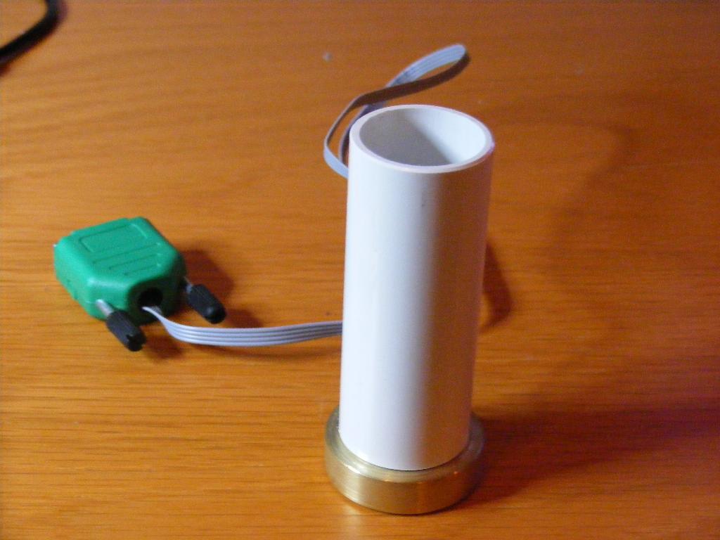
Accelerometer
This object handles an accelerometer, which delivers
its results as pulse widths.
Accelerometers never measure
acceleration only. They measure the sum of acceleration
and gravity, i.e. they measure one component of this
vector. Hence, if the accelerometer isn't moved very
vividly, it can be used to measure tilt. When the
accelerometer is tilted, a no longer horizontal accelerometer
will measure a component of the vertical gravity vector.
I used this to make a simple joystick. It has a vertical
plastic tube with a horizontal accelerometer mounted between
some foam rubber pads. At he bottom of the tube, there
is a heavy plane brass foot. If you leave the joystick
on the table, it will show nothing (except some bias), but
when you grab and tilt it, it will show the tilt angles.
The object contains a censor function
which eliminates sudden spikes in the signals. Biases
can be eliminated by calling the acc.cal function
in a situation, when the accelerometer shouldn't show
any acceration (the joystick resting on the table).
The signal is scaled as a number between 0 and 4096,
with 2048 representing zero signal.
- acc.init initializes the software, by
setting the pin numbers. Call as xpin ypin [acc.init].
- acc.get brings the two acceleration signals
to the stack, with the x-acceleration highest.
acc.get uses acc.scalex/y and acc.censor to scale
the signals, and filter out sudden spikes ("outliers"),
- acc.cal removes bias. Call as
ax ay [acc.cal] where ax and ay are
current or recent readings of acceleration, in
a situation, when the accelerometer should show
zero outputs.
Download acc.myo
Download num.myo
Odometry
Odometry comes from a Greek word for "way" or "road",
and it is the art of determining travelled distance.
To do it we have a striped strip and two optical sensors.
We can put that strip around a wheel of a robot, to measure
its travelled distance, or we can glue the strip on the
road itself, that we travel along. Here's how it works:
We have two pictures of a strip and two optical sensors
(the circles) in both pictures. The strips move as
indicated. In both these cases, the right hand detector
switches from white to gray, which indicates a motion. But
which motion is it, the upper or lower case? We can tell
by looking at the left hand sensor. In the upper case
it is white, in the lower it is grey. So now we can
detect a motion "with sign", and we can accumulate the
incremental motions to a distance travelled.
The Odo object odo.myo handles two strips and two sets
of optical sensors, to determine movements in the plane.
- odo.init. Call as
y2pin y1pin x2pin x1pin [odo.init] with
pin numbers for the different sensors.
- odo.odo pushes the two position
coordinates on the stack
- odo.reset resets the accumulated
positions coordinates to zero.
The odo object is used in the
The Milling Machine.
Download odo.myo
Proto zigbee
These objects control IEEE 802.15.4 modules. Read about
them here.
The basic object is zig.myo, which contains
the following functions.
- z.init initializes the object. Call as
zinpin zoutpin [z.init], where zinpin is the
pin connected to the receiving pin of the zigbee
module.
- z.initin is used when zigbee is only used
for receiving data. In this way one is not forced
to set a computer pin as an output pin.
- z.ssend sends a string over zigbee. Call
as address [z.ssend] where address is the
address of the string. At the end of the string,
there shall be the ascii code for the null character,
i.e. the number zero (Null terminated string).
- z.bsend sends a single byte over zigbee.
Call as byte [z.bsend]
- z.cr sends a carriage return over zigbee
(ascii code 13). Call as [z.cr]
- z.rec receives a single byte over zigbee.
The function is blocking, but will return the byte
on the stack, once it has arrived.
zigread.myr is a simple program to demonstrate how
to configure a proto zigbee module. It is a stand alone
program, that doesn't use any object file. You have to
set the pinnumbers to the zigbee modules. This must be done
in both processes. One must also set the current baud rate
of the module. The modules are delivered with a baud rate
of 9600. This program changes baudrate to 115200 (which
you perhaps want). The next time you run the program,
you thus have to change the default baud rate to
115200.
The program has two processes, one that sends commands
to the zigbee module, and one that captures responses
from the zigbee and sends them further to the PC. On
the PC, you may run Parallax' serial terminal or a standard
Hyper Terminal to see the result.
You command the module with so called AT-commands, which
start with the characters 'AT'. To make the module accept
these commands, you have to make it leave its transparent
mode. This is done by waiting 1 second, sending the
code '+++' and then waiting 1 more second. We send
a code for reading the current baud rate, then we change
the baud rate to 115200 (code 7), and then we verify the
change (a response of 7 shall appear on the PC). Then we
just verify that the zigbee channel has its default value
of 12 (hexidecimal C). Then we check the PAN-ID, and
whatever it is, we set it to 5. We wait a while and then
verify. Then we write the modified data to the module's
EEPROM memory. Finally we return to the transparent mode.
Download zig.myo
Download zigread.myr
FM radio
This objects controls a little chip, AR1010,
which contains a complete FM radio in a chip,
4 x 4 mm in size. The chip is controlled from
a computer, and the object contains functions
for that. We will however describe all the details
about this in the FM radio application.
Linear Camera
The linear camera is a camera that produces an
image, 1 pixel high and 512 pixels wide. We will describe
the functions of this object, while we describe
the Linear Camera Application.
Applications
A "Universal" Computer
Once I made a box containing a Propeller Computer,
A/D converters,
a bluetooth modem, an alphanumeric display, an SD card
reader and three power amplifiers. Unfortunately the
box became full of wires, and it wasn't easy to keep all
these wires intact.
So here's a more modest project. It is a smaller box
which contains a Propeller computer together with the
normal EEPROM and the normal 5 MHz crystal, an A/D
converter, an RGB led for debugging etc., and circuits
for voltage supply. Here's what the circuit board looks
like:
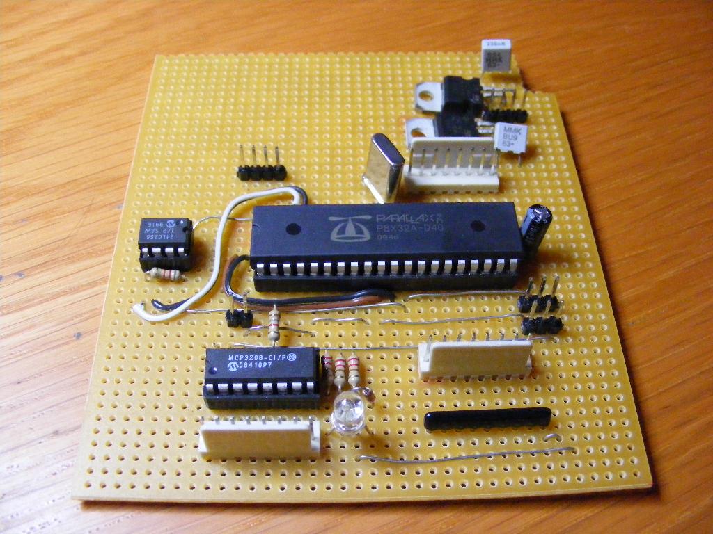
Here's how the circuit board is connected to external
connectors. I have always liked to use 9 pin D-sub
connectors.
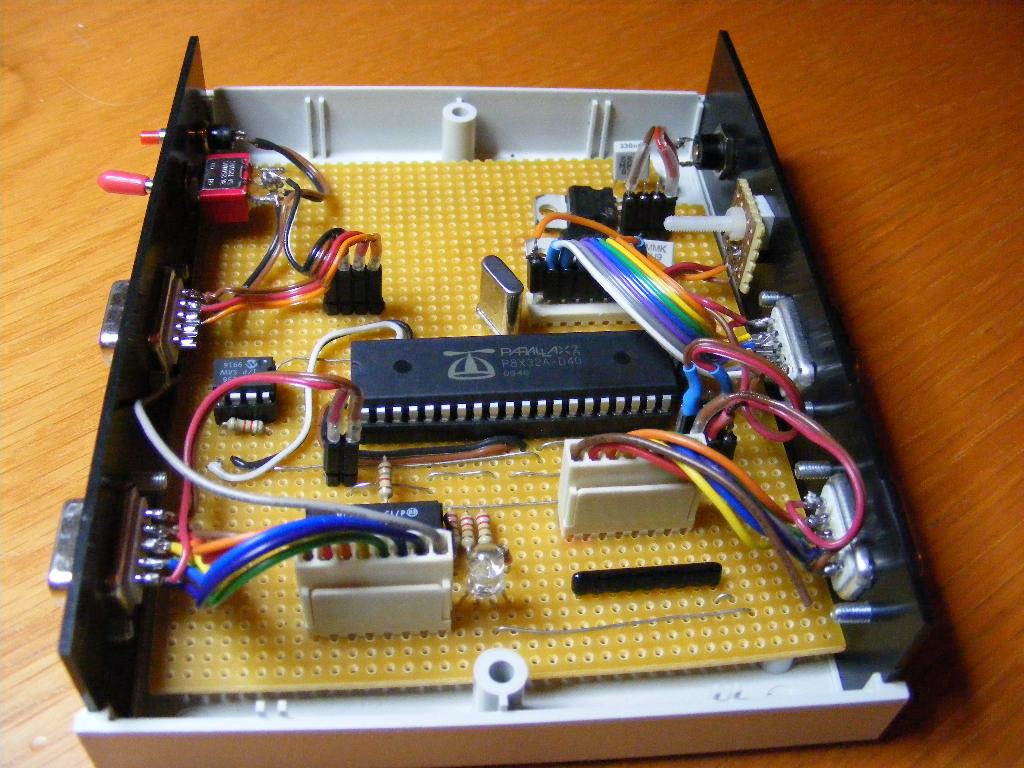
On this side there is a reset button, and a switch which
disconnects the reset input from the PC connection. This
is necessary if you want to send data from the PC, without
resetting the computer every time. In the middle there
is a programming connector. I only use 4 of the connection
points there, and they go directly to the pins of a
Prop Stick device, that I have built into a D-sub connector
with housing. The right hand connector goes to 7 of
the 8 analog inputs of the A/D converter. The remaining
two pins of the D-sub connector go to ground and 5 volts
supply. To the right on the top of the box, you can
see the end of a plastic screw, that acts as a ray guide
from the RGB-led.
On this side there are connections to 14 of the universal
digital I/O pins of the Propeller. The left connector
also has a ground connection and a connection to 3.3 volts.
The right connector instead provides ground and 5 volts.
Further right there is a small handmade connector for
connection of the alphanumerical or graphical displays, which
are housed in separate boxes. Rightmost is the supply input
which receives an unstabilized voltage of 7.2 to 12 volts.
Bluetooth has been replaced with Zigbee, but the Zigbee
modem is now placed on a D-sub connector. The power amplifiers
are built into a separate box of the same shape as the
computer. As mentioned, the two displays, the alphanumeric
and the graphic, are placed in separate boxes.
The Robot
Everybody who has a Propeller, or any other microprocessor,
wants to make his own robot. Here is mine:
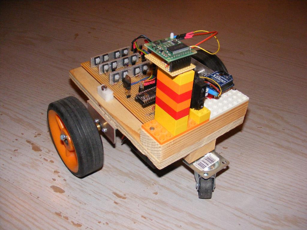
It has two relatively strong 12 volt motors with gear
boxes (1:21), two strong rubber wheels and a caster wheel
in front, and a led battery, that I charge with a CTEK
led battery charger.
It has three power amplifiers. They
are built with discrete components, but they don't work
at very high PWM frequencies, as they get hot. It's OK
for this application to work with low frequencies, but I
don't recommend these amplifiers. The alternatives mentioned
previously are better. Anyway, you can see the coolers for
the transistors as three aluminum bars on the circuit
board.
The computer is a Spin Stamp, which is a surface mounted
Propeller mounted on a hybrid circuit, which also contains
a crystal (10MHz unfortunately, perhaps), voltage stabilizers,
and an EEPROM. On the card, there is also a 3208 A/D converter,
and two voltage stabilizers. One of them reduces the 12 volt
battery power, not to exhaust the stabilizers on the
Spin Stamp. The other provides 3.3 volts for some sensors.
Unfortunately, the Spin Stamp doesn't make its own
3.3v voltage available externally.
In the front, there is a Lego block, on which I can put
sensors and other stuff, mounted on small Lego blocks.
In the picture you can see a compass, mounted on a high
Lego tower, to keep it away from the magnets of the
motors, an infrared distance sensor, and a "proto Zigbee"
unit. The whole robot is controlled over proto
Zigbee from a remote control. I also have an infrared receiver,
adapted to an infrared LED modulated to 38 kHz with a
Propeller computer. So, there is an infrared control for
the robot, but it requires that you direct the LED
pretty accurately towards the receiver.
One thing I don't have is odometry sensors on the
wheels. I once had that. You can read more about
that in the description of the
milling machine.
I am a specialist in autonomous control of unmanned
vehicles, but as this is a hobby, I have made a robot
completely free from all autonomy. It is a remotely controlled
vehicle, basta!. But I did some experiments with a
software, that would drive the robot to the nearest object.
But that is not ready yet.
Otherwise the robot is pretty robust, fast and strong,
though it can't compete with modern radio controlled model
cars with brushless motors.
Here's the software
RobotZ.myr
The first thing you notice is a "10 MHz" tag. That's
because the Spin Stamp has a 10 MHz crystal, while the
standard is rather 5 MHz. The Spin code, that is generated
from the Myra code has to know that. So the Myra code
uses the "10MHz" tag to modify the Spin code.
The process input receives the input from the Zigbee
unit. It's a single number comm whose bits
signal which buttons on the remote control are pressed.
The process motor's main program decodes comm
and sets two motor masks and a velocity. The motor masks
are each of two bits, and determine whether the motor
will run forward (01), backward (10) or be stopped (00).
The velocity is set lower if we turn the robot left
or right, and higher when we drive forward and backward.
This facilitates the driving. In the main program, there
is also a call to a heading control function, heading,
which drives the robot to
a given heading, as measured by the compass.
The motor is finally controlled by the function
drive. It sets the PWM duty cycle according to
v (16 is full speed, 100% duty cycle). The motor masks
merged together with shifts and an or instruction are
sent to the amplifiers during the on period, and 0 is
sent during the off period. The total cycle time of
the PWM signal is 80000000/100 ticks, which gives a
repetition frequency of 100 Hz.Fortunately we don't
hear any 100 Hz tone from the motors, probably
because of the inertia of the wheels.
The compass process catches the signal from the
compass, which amounts to measuring the length of a
pulse, that the compass electronics sends regularly.
The scaling i 100μs/degree.
Finally a word about the heading control function
heading. The control error is basically
psi - psiC where psiC lies on
the stack, and the measured heading is a global
variable. But just subtracting angles is a little
dangerous. 1 degree and 359 degrees are only 2 degrees
away from each other, but the subtraction would
give 358 degrees. So we have to "normalize" the result to
within ±180 degrees, by adding or subracting an
appropriate multiple of 360 degrees. Then we control
the motor mask with the sign of the control error,
and we control the velocity with a ramp function of
the absolute error. (We use the || assembler function).
The ramp function is difficult to trim, due to the
friction of the motors. The motors don't run at all
if the signal to them is too low. That is also why
I haven't succeded yet with my "drive to the nearest
object function".
The remote control
The remote control is a box with buttons, a Propeller
computer with its crystal and EEPROM and a proto Zigbee
unit. It is driven with a 9 volt battery. At the back
side there is an on/off switch and a programming connector.
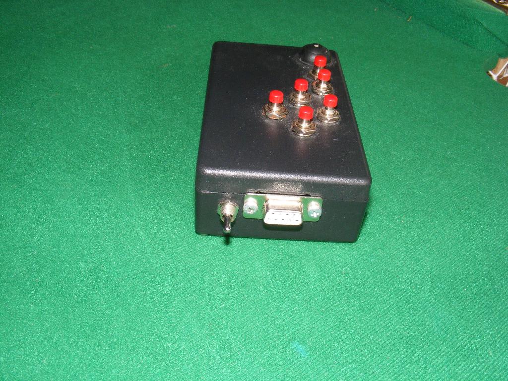
There are 7 buttons, which is less than 8, so the whole
button pattern can be sent in one byte. For that, each
button is connected to its own Propeller input pin.
Download remote.myr.
Download zig.myo.
The Wheel Steamer
This picture shows the wheel steamer
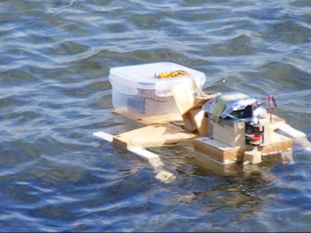
I built it together with my son, when we were in the country
with limited technical resources. You can see, perhaps,
that we are not exactly any expert naval architects.
The ship is built in fur wood, and not plastic foam, so
it is rather heavy. To keep it afloat, it is not a katamaran,
but a pentamaran.
We found a small DC-motor as a main motor. To keep it away
from the water, you can have a propeller with a long shaft,
or a belt drive. But a wheel steamer was also a way to
bring the motor up. We have only one drive wheel, placed
in the middle of the ship, and built around a square hub.
Control is made with a rudder, which is driven with a little
gearbox kit (for those who want to learn what a gear box is).
It gives a slow enough movement to make the rudder
controllable.
We also found a waterproof lunch box, in which we mounted
the electronics, which consists of a proto Zigbee module,
a Spin Stamp module, and a TDA2050 based power driver.
I don't publish any software here, as it is essentially the
same as the software for the robot, although we have one
drive wheel and a rudder here, while the robot has two
drive wheels and a passive caster wheel.
The Milling Machine
I am the happy owner of the milling and drilling machine
you can see here:
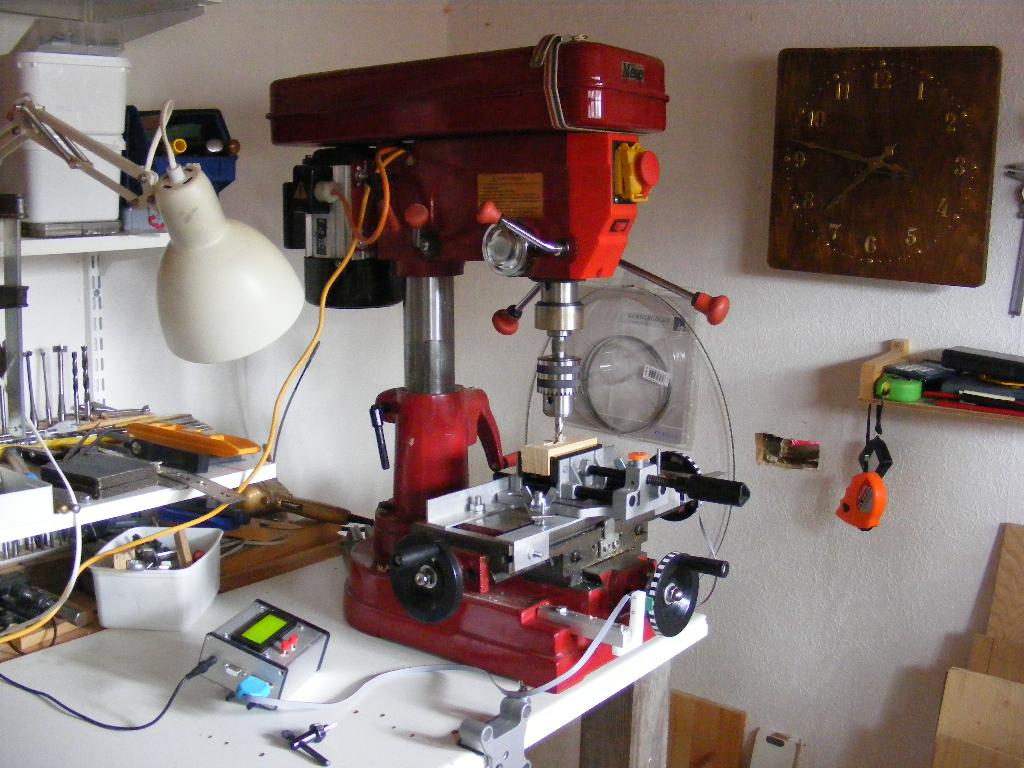
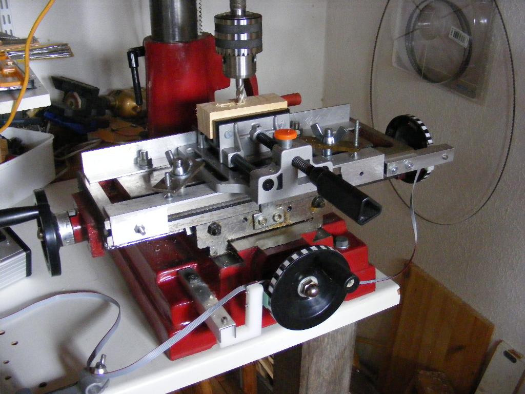
It has a coordinate table with two cranks to move the
workpiece in two orthogonal directions. I have mounted
striped tape on the two cranks, and then I have mounted
a pair of reflex detectors nearby. The reflexdetectors
are from Polulu and intended for odometry. The following
pictures show the arrangement more in detail:
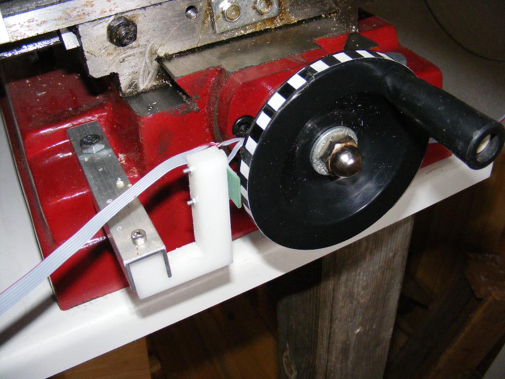
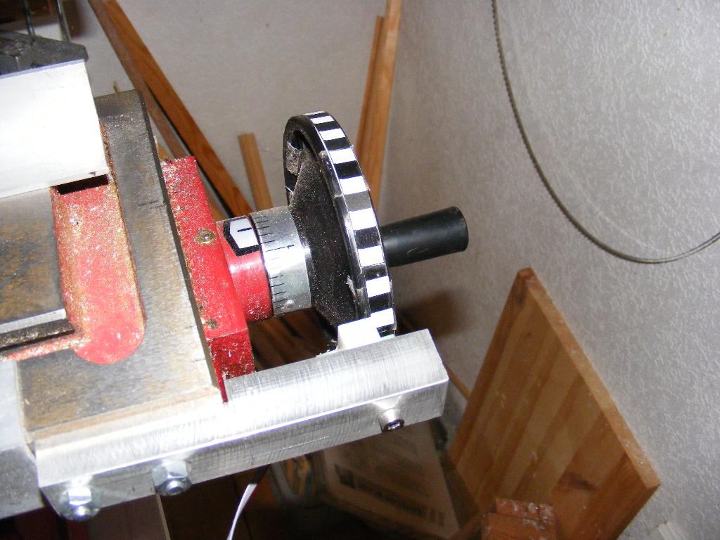
Then i have coupled the reflexdetector to a box containing
a Propeller computer and an alphanumeric display.
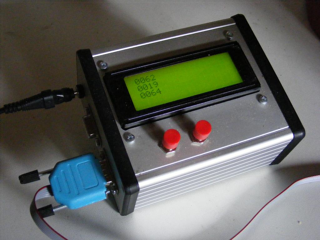
The software consist of odometry computations based on
the odometry object as described above. With the stripes
I have made, the resolution in table movement becomes
1/14 mm, but I have recalculated this, so that I get
resolution of 0.1 mm. On the two first lines of the
display, I show the coordinate table positions in
tenths of milimeter. All coordinates refer to a reference
point, that you set by going there, and then pressing
the right hand red button.
The third line shows the distance to the referenc position.
This is computed with Pythagoras' theorem and the
num.itsqrt function for computing the square root.
This function is of course usefull when you want to mill
out a big circular hole. If the hole should have the radius
R, and your milling tool has the radius r, you should move
out to the distance R-r everywhere, but no longer.
Another thing that you maybe would like to mill, is an
oblique straight line. You could define such a line by
moving to two points on the line, and press the two
red buttons. Then the display could show the distance
to the line. This is a function I haven't made, but it
would be possible.
The equipment is good for milling, but also for drilling where
you could place your holes with good precision. In all,
this is a very nice little equipment, that raises the value
of the machine considerably. Of course, from this point one
can go on and add motors, and make a numerically controlled
machine.
The following picture gives a little instruction for how
to make a hole for a D-sub connector.
 Download Odo.myr
Download Odo.myo
Download Num.myo
The USB oscilloscope
FTDI manufactures some USB modules, where data to be
transfered are loaded in parallell, one byte at a time,
rather than serially. On the PC side, data appear in
a VCP port, which makes data available one byte at a
time, or over D2XX. With this type of module, data can
be transferred faster than over RS232 emulators.
The module can handle the situation, that the USB bus
is busy, by stacking up non sent data on a stack
(a FIFO stack, First In First Out).
I have used this module to build a data logging system,
with data display on the PC side, a so called USB
oscilloscope. It works in two modes, a digital mode
where one or more digital signals (being either 1 or 0)
are transferred, and an analog mode where one or more
analog signals are transferred. The advantage of the
digital mode, is that it can sample data faster.
In digital mode, I can transfer 300000 bytes/second.
The byte can contain up to 8 digital signals, which
are read directly from the computer input pins. I have
preferred, though, to use the 8:th bit for time marking.
The last bit flips every 1ms with high precision. This
allows me to create a very exact time scale on the PC
side. Furthermore, I have chosen to pull out only
two digital signal wires from the computer, but that
is easy to change.
In analog mode, I have two operational amplifiers,
to scale the inputs, and give them a symmetric range
around zero volts, and then I use two channels of
an 8 channel 12 bit A/D-converter (Microchip 3208).
I make the A/D conversion, and the packing of data into
bytes in one processor. A second processor handles the
USB device. An analog data takes up 12 bits, and I pack
that into two bytes. That leaves 4 bits free. I use
the last bit for time marking, as in the digital mode.
The remaining 3 bits contain the fix code of 101. The
PC uses this, to recognize the least significant byte,
so that it doesn't loose phase, and mixes the two bytes
up. This describes how I handle 1 analog signal and
two bytes, and that is what I do right now. With two
analog signals, I have to reduce the sampling rate to
one half. In analog mode, I transfer data at a rate
of 66.666 kHz, but not all these data are new analog
samples.
For both modes, there is a red trig button. Its signal
is also pulled out, to admit electronic triggering.
When the trig signal comes, 50000 data are transferred
to the PC. Then the signals can be analyzed with
an interactive plot program. There are different programs
in digital and analog mode. In the digital mode, one
sample covers 0.168 seconds of real time, in analog
0.75 seconds.
The fundamental principle here is one time triggering.
You get one set of 50000 samples, to analyze afterwards,
unlike a conventional oscilloscope, where you retrigger
all the time, which gives you problems, when you have
non periodic signals. Here, the problem is to trigger
at the right moment.
The signals enter the oscilloscope through a 9 pin
D-sub connector. At these frequencies there is no nead
for high quality coaxial connectors. There are two
probes, one for digital mode and one for analog mode.
The software distinguishes the modes through a jumper
wire in the digital probe. Then you have to select
the corresponding software on the PC side. On the
Propeller side, there is only one program, but if you
change probe, you have to restart the device.
Here is a drawing of the electronics:
You can see the standard set up of a Propeller with
crystal, EEPROM and prop plug. In the upper left
corner you see the connection of the 3208 A/D converter.
As it is connected to other pins than the normal
you have to use the parametrized initialization
init_analogp. The lower left part of the drawing,
is the analog part of the system. We come back to
that in a while.
In the upper right corner, there is the connection
of the USB module, with the USB connector depicted as
a gray square. The module is such, that you have to
connect ground and power to a number of places externally.
With the way it is done here, the whole apparatus will be
fed from the USB output of the PC. There is also
a 3.3 volt input, to make sure that the module outputs
are constrained to 3.3 volts, so that the Propeller
inputs are not destroyed. The 8 data pins are
connected directly to the Propeller outputs 0 to 7.
Then there are four control pins, which go to the Propeller,
The Propeller software will handle these pins
apropriately.
Download fifo.myr.
This is a simple program, that, depending on mode, uses
the two assembler functions fifolog or fifoalog.
These refer over the stack to the variable tstamp,
which is the time marking signal, or x which is
the word to transfer. It would seem natural that the
references here would be through adresses #tstamp and
#x, but these variables are variables in the common
variables, and such variables are always transferred via
adresses, that are used in rdlong instruction. It
would be neater, if we could write #tstamp and #x, but it
would be difficult to use that in the assembler functions.
Otherwise, fifolog and fifoalog are simple 50000 times
loops.
Here are some hints about the analog circuitry at the
lower left of the diagram. To create a symmetric range
of the analog input, we need a negative reference voltage.
We use a chargepump, MAXIM 660 for that. The operational
amplifiers are of type OP90. They can be driven with
a single 5 volts supply, and they produce output "rail to rail"
i.e. from 0 to 5 volts. The trim potentiometer should be
trimmed, with the input disconnected or grounded, so that
the output i exactly 2.5 volts. This is the middle of the
A/D converter's range. Hence the ouput will be 2048. This
number is then subtracted on the PC side, so we get zero
output for zero voltage. Now, nominally, the trim pot value
should be 390/2 = 195 kΩ. The all over impedance at the
input is then 390/3 = 130kΩ. So if you let R be 130 kΩ,
you get a gain of 1, and a range of ±2.5 volts. You probably
prefer a range of ±5 volts, so you chose 260 kΩ. This
is also the input impedance of the device. It is not so
impressive, but probably good enough for most purposes.
If you trust the precision of the 390kΩ resistor and R,
you trim the bias and the gain at the same time with
the trim potentionmeter.
Information and download of the PC java programs is
found here.
The Data Logger
The data logger makes the same job as the USB oscilloscope,
but without a PC. Instead data are shown on a graphical
display. The device is controlled from a standard
PS/2 keyboard.
Data are stored in a, 4096 words wide, data area in the
common memory, by means of an assembler routine logg.
Data are displayed with a program in the graf object (graf.myo)
called gr.loggshow. It makes a pixelmap in the standard
way for the graphical display in an area in common memory
called gr, 256 words wide. This is then transferred
to the graphical display for final drawing. gr.loggshow
is controlled by 4 variables. The scaling in the horizontal
and vertical direction is made as shifting an integer number
of steps according to the variables tshift and
fshift. The curves are also moved in both directions,
so that the left hand edge corresponds to a time tstart,
and that the low edge corresponds to a value flow.
These parameters are controlled from the keyboard.
The keys used, have the following meanings:
- G(o): Start collecting data
- I(n): Move into the curve, by scaling up time.
- O(ut): Move out from the curve, by scaling down time.
- F(orward): Move forward through the curve.
- B(ackward): Move backward through the curve.
- U(p): Move up through the curve.
- D(own): Move down through the curve.
- N(ear) Scale the curve up in the vertical direction.
- M: Scale the curve down.
Download Logg.myr
Download Graf.myo
Download Key.myo
The process logga logs data into the area
logspace. The assembler function initlog receives the
starting adress of logspace and the size of the logspace.
The assembler function logg receives the data
to log, logs the data, increments the adress, and
decrements a counter from the size of the logspace and
returns its value on the stack. logg is called
until that counter is returned as 0. Then logga
goes back and waits for a new start signal. What we
logg here is a signal from an A/D-converter channel.
The process draw draws the plot based on the
parameters tshift, fshift, tstart
and flow. When a draw has been made, the
image is sent over to the display computer by the
process sendim based on the variable imsynk.
The keyboard is read by a separate proces keyread,
which does nothing else.
Then, the keyboard is interpreted in the process
keycontrol, which sets a start signal and
the parameters tshift, fshift, tstart and flow.
Here is a picture of the setup with a potentiometer,
whose signal is logged (The one with a red and black knob).
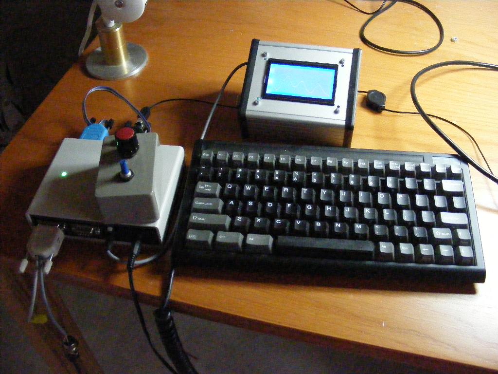
Here is a logg:
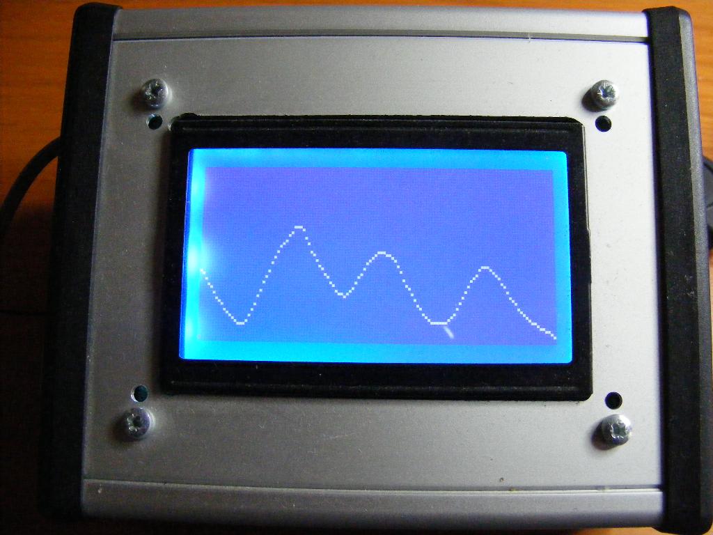
Here I have zoomed into the first peak:
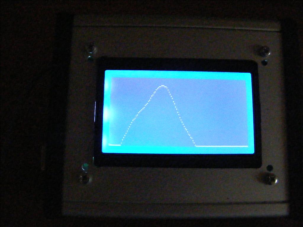
The Telescope
When you look at a star with a telescope, the telescope
will rotate with the rotation of the earth. So to get a
stable picture, you have to rotate the telescope backwards,
relative to the earth. Amateur telescopes usually have
something called an equatorial gimbal system, which is
a mechanical arrangement, such that one of the degrees
of freedom falls along the rotation axis of the earth.
There is a knob there, and by rotating that slowly, you
can counteract the rotation of the earth. Equatorial
gimbal systems are a bit clumsy, though. They require a
big counterweight, which makes the whole telescope heavy,
and the telescope tube sometimes makes a pretty awkward
journey, when you direct it against different parts of
the sky.
So the whole project here is about making a virtual
equatorial gimbal system. The starting point then,
is what I would call a "fork gimbal system". The telescope
tube is hung up between the arms of a fork, and can
be moved up and down there. This is called the elevation
movement. Then the fork can be rotated around a vertical
axis. This is called the azimuth movement. The problem
now is to distribute the counterrotation against the rotation
of the earth to the two axes, azimuth and elevation.
Here is a picture of the fork gimbal arrangement:
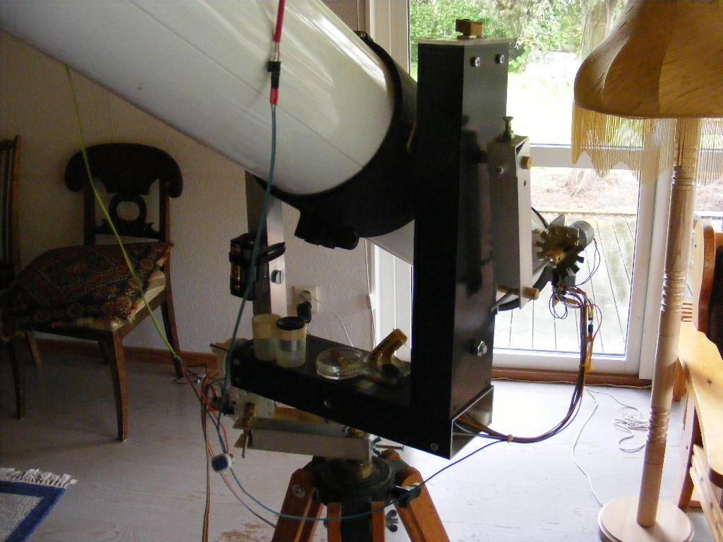
First of all, the rotation of the earth is directed towards
north, and it is tilted up from the horisontal plane with
the latitude of the place. So on the equator, the rotation
axis is lying down, and at the North Pole it stands right up,
so the direction towards north doesn't matter, which is lucky,
because there is no notion of north at the North Pole. Then,
there is a more tricky mathematical problem. The azimuth angle
and the elevation angle are so called Euler angles. There is
a third Euler angle around the axis of the tube. So what we
want to control is time derivatives of the Euler angles,
and what we have is the earth rotation vector. But the
relation between rotation vectors and Euler angle derivatives is
a little bit involved, and it is easy to make mistakes there.
But I provide you with a Java program that solves the problem.
The result shall be a function with three inputs:
- The latitude of the place.
- The elevation angle
- The azimuth angle, measured relative to north
... and two outputs
- The time derivative of the elevation angle
- The time derivative of the azimuth angle
The motions involved are very small. The earth rotates
1 full revolution in 24 hours (or to be more exact,
366.25/365.25 full revolutions in 24 hours). We can not
hope to use a speed servo to achieve such small motions.
Instead we work with small fixed angle increments. The
Java programs produces the time interval between these
incremental movements. Concretely the Java program produces
a definition of an array written as Myra code. This
Myra code is then copied into the complete Myra program.
The Java program assumes one latitude angle, which is the
latitude angle where I live. If you don't happen to live
at the same latitude, you should change the lattitude
angle. Furthermore, the azimuth angle rate is virtually
constant in elevation and azimuth angle. It is essentially
the vertical component of the earth rotation vector. In my
system this rotation corresponds to an interval between
incremental movements of 3.4 seconds.
In elevation, the angular rate varies with both azimuth
and elevation. When a star is seen strictly south, it doesn't
move in elevation. It is on its peak on the sky. To the
left of south (i.e. east) the stars are moving up with
varying speed depending on elevation. On the right side of
south, they move down, and so should the elevation angle.
These effects are seen in the table.
Negative elevation motions are encoded as negative time
intervals. The Propeller program has to observe this, and
use the positive time interval, but at the same time
reverse the motion direction.
Technically the angular increments are made with a combination
of a motor, a hole disc, an optical fork, a long scew and
a leverarm with a threaded joint. In the computer there is
a motion state variable called x (xel for elevation
and xaz for azimuth). x flips between 1 and 0, once for
each time interval. When x is 1 the motor moves until light
passes through the hole disk. When x is 0, the motor moves
until no light passes through the hole disk. The hole disk
has 12 holes. Consequently the disk moves 1/24 of a whole
revolution per x-flip. This makes the screw threading move
outwards or inwards 1/24 of 0.5 mm (because it is a M4 screw).
This pushes the lever arm outwards this much, and as it
is a 1 dm lever arm, the angle increment is:
1/24·1/2/100 radians = 2.08333·10-4
This value appears in the Java program.
Here is a picture of this arrangement in azimuth. I painted
the hole disk with opaque color to avoid reflexes, but it
turned out to be unnecessary.
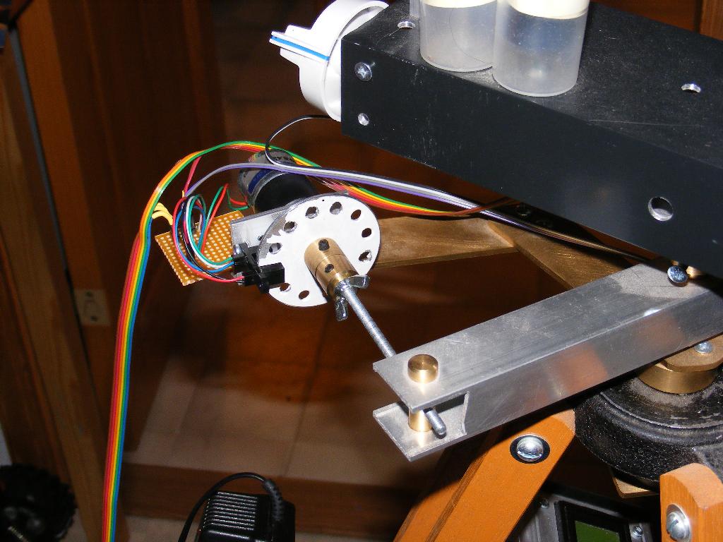
You can see the motor, the hole disc, the optical fork
(in black), the screw, a threaded joint in brass, and
the lever arm in aluminum.
This is the correspoinding arrangement in elevation.
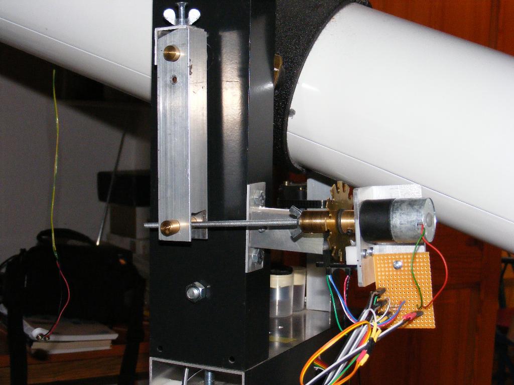
The
disc is slotted rather than a hole disc, which makes the
mechanical mounting of the optical fork a little easier.
You can also see the arrangement that locks the lever
arm to the elevation axis of the tube, with its wing nut.
Inside the aluminum tube profile, there is piece of brass
with an oval hole, which is pressed towards the elevation
axis.
It is worthwhile also to have an electric focusing. If
not, you have to touch the oscilloscope focusing knobs,
and it is hard to make the gimal arrangement so stable,
that it doesn't shake a little. Focusing is something you
have to do, after you have changed ocular. Fortunately
I have two amplifiers left for driving a focus motor,
and i have two buttons left on the remote control. The
software is simple, but of course you have to find out
how to couple a motor to the focusing knobs. This
picture shows how I have done it:
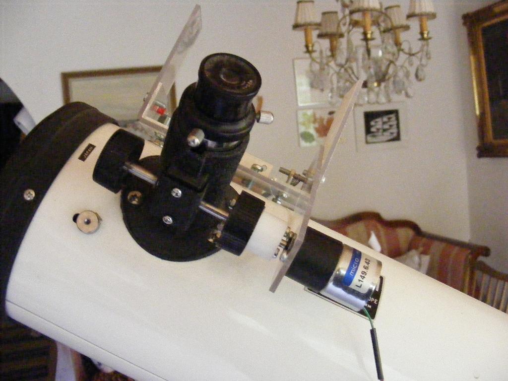
The computer has four input signals. Azimuth and elevation
signals come from potentiometers. They are right now handled
manually. The user is supposed to direct the elevation
potentiometer parallell to the telescope tube. A link arm
could make this automatic. The user is supposed to direct
a bar fixed to the other potentiometer to the south. An
electronic compass could do this, provided it would be
calibrated. The other two signals come from the optical
forks. All these signals are fed to the A/D converter.
The output from the computer is three pairs of motor signals
connected to the two poles of the three motors through
power amplifiers. The amplifiers are made with
IR2103 FET drivers. Six such amplifiers
(good to drive three motors) are built into a box. They
interface to the computer through a shift register, which
would allow a two wire serial interface. Here, however, we
use a parallell interface by setting the shift register in
parallell mode. It still needs a clock signal to move
the computer signals to the amplifier inputs.
Now we think of motor control as setting a six bit code,
which controls all three motors.
A code of 101010 would drive both motors forward.
A code of 000100 would hold the first and third motor and drive
the second motor backward etc. The toggle process
sets these codes based on the state variables xel an xaz,
and the fork positions. In turn, these computations rely
on the time intervals dtel and dtaz, and on the directions
direl and diraz.
The process motor sends the code further to the
amplifiers, which amounts to shifting the codes to the
right pins, and clocking the shift register. It also has
to satisfy the amplifiers requirements to get zero input
now and then.
The times dtaz and dtel and the directions diraz and direl
are computed by the times process, which contains
the table from the Java program. In fact dtaz and diraz
are constant. The computation of dtel is based on a table,
where azimuth and elevation have been discretized to
tens of degrees.
This discretization is made in the anal process
together with the A/D conversions. The discretization of
the elevation angle is based on measurements. The optical
forkpin signal are discetized to boolean values, using the
G assembler function, which maps any number greater than
0 to boolean true (1) and any other number to boolean false
(0).
Finally, there is a manual control of the telescope from
the standard remote control used for the robot. The remote
control signal
is received through Proto Zigbee and is called comm. It is
a mapping of the buttons pressed, and it requires that
only one button is pressed at a time. The manual
process computes motor codes similar to those from
the toggle process, and they also control the focus motor.
If no elevation button (the upper and
lower) are pressed, an ignore code is set. Similarly the
azimuth motor code and the focus motor code can be set
to ignore. The merging of
the "automatic" motor codes codeel and codeaz, and the
manual ones, mcodeel and mcodeaz is done in the process
toggle. If a manual code is not ignore, then it overrides
the automatic code.
Download Teleskop.myr
Download Display.myo
Download Telskop.java
Download Text.java
(used by Teleskop.java)
Here is finally a short manual to the telescope:
- Make sure that the lever arm threaded joints
are in appropriate positions along their screws.
The azimuth joint could be towards the end of the
screw (It will move inwards).
The elevation joint could be near the middle
of the screw. Arrange this with the remote control.
- If you feel you want a cup of coffee, or expect
that the next step will take some time, disconnect
the power to the electronics.
- Loosen the gimbals from the lever arms.
In elevation you could see a wing nut for
that in one of the pictures above. There is a
similar wing nut for the azimuth.
- Direct the telescope tube to what you want
to look at using the manual sight on the
tube. When ready, tighten the lever ams to
the gimbals again.
- Align the elevation potentiometer along the
telescope tube, and direct the bar on the
azimuth potentiometer towards south.
- Reconnect the power to the electonics.
- Look in the telescope ocular, and if you
see your astronomic object there, center it
with the remote control. Otherwise you have
to scan around with the remote control to
try to find it. This can be quite difficult,
so you may prefer to go back and use the
sight on the tube instead.
- Once the object is in the center, it will
stay there for a good while. You may have
to adjust after a while with the remote control.
- Now you can also start changing ocular to
get a closer look, and you can do that without
having to worry where the object goes while
you don't observe it. It stays where it is.
- After more than a good while, you will have
run out of threading of your screws. No more
to do than to go back to point 1 again.
The FM radio
This radio is based on a chip from Airoha called AR1010.
In a volume of 4x4x1 mm it contains a complete FM radio
with stereo decoder, sound outputs and two different
computer interfaces. I don't know if this is a so called
Software Defined Radio, i.e. a completely computerized
radio, or if there are any special circuits. Nevertheless,
you don't see any traditional things like coils or capacitors.
My work is based on a small breakout board, which includes
a crystal. It is sold by Spark Fun Electronics. Apparently
Telefunken has made circuits of this type, and there is
another chip called SI4375, which also has a short wave
band, but it seems to be sold by nobody. This will
change perhaps.
The problem with Airoha AR1010 is that the documentation
to it is confidential!. All that is availble is a
datasheet that describes the electrical connections, but
it says nothing about the protocols, with which you speak
to your radio chip. A software specification is avaiable on
the internet, however,
though it is pretty hard to find. The name of the document
is ar1000F_progguide-0.81.pdf, which you can try on Google.
One adress you find is www.docin.com/p-34190202.html which
is a chinese site where you can see and read the document,
but it is unclear to me how to download it. I have downloaded
the document, of course, but I don't dare to make it
available here. Some people have complained about the
quality of this document, but I think it is quite good.
As you can see from the name, it is actually about the
circuit ar1000, which is a more advanced sister to ar1010,
which has RDS, but it works for ar1010 also.
The breakout board is maybe intended for surface mounting
on a circuit board, but it is easy to connect to a normal
hole mount board with some small wires. The breakout board
hides some details of the original cicuit, so all you
have to think about is this:
- Ground and Power supply (2.5 - 3.6 Volt)
- Antenna input
- Sound output (2 stereo channels)
- Four connections for interface to the
controlling computer.
If you ground the Busmode pin in the computer interface,
you get I2C interface, and then all that remains
is a clock pin and a data pin. We have mentioned about
the I2C interface here,and
here will come some more detailed information.
The AR1010 chip has 18 registers, each with 16 bits, and
you control the radio by writing into these. The procedure for
this is the following:
- Send an I2C start pattern
- Send the adress of the chip, which is
hexadecimal 10, but this should be followed
by a 0 write bit, so what you send is actually
hexadecimal 20 (in one byte)
- Send the number of the register, you want to
write to.
- Send two bytes of data, to fill the sixteen
bits of the register.
- Send an I2C stop pattern
The I2C start pattern means that you set
the data pin and the clock pin to zero in that order.
Now, the data and clock line have low impedance,
which means that the master has taken control over
the bus.
The I2C stop pattern means that you set the
clockpin and data pin to one in that order. After that,
the master has a high impedance output, which means
that it refrains from the bus till further.
On the assembler resource file there are assembler routines
for start stop write and read. With a similar pattern
as above, you can also read any register, to find out
about the status of the radio. I found that unnecessary.
I trust that the radio will do what I tell it, and I
expect that the corresponding status bits will be set, if
I just wait a while.
The programming guide describes the contents of most of
the registers, but it is obviously an incomplete description.
There is a set of default settings to all the registers, and
sometimes you set bits to registers that, according to
the description, don't mean anything. Anyway, the default
settings work fine. There is one set of default settings
if you have a crystal on the chip, and another if you set
the reference frequency from your computer, but here we
do have a crystal. To initialize the radio you should set
these defaults from register 1 and up, and last to register
number 0. You will find the default values, and how
to initialize the radio in the file radio.myo.
The rest of the settings have to do with setting frequency,
setting volume, muting and unmuting.
Radio.setfreq receives the frequency in 1/10s of MHz. This
is also how the frequencies are distributed to the users.
If you want to transmit something on the FM band, you are
assigned a frequency in MHz with one decimal. So if you
hit that frequency in the receiver,
which you should be able to with
a crystal, you should be exactly tuned. If you multiply
the frequency with 10, to get an integer, and subtract
690, you get something called a channel number.
That channel
number should go into register 2. You first write into a
mirror of that register in the computer, and
then send that mirror over to the real register. But
you also have to toggle a so called tune code. The
radio retunes, when the tune bit switches from 0 to 1.
Before and after frequency change, we mute and unmute
the radio, to avoid some noise. This is done by setting
mute and unmute codes to register 1.
Volume is set in radio.setvol which receives a
volume number between 0 and 15. For some reason, the volume
scale is turned up side down, so you should send
(15 - volume) to the radio. This volume should be sent to
register 3. There are some less significant bits for volume
in another register. The programming guide shows how you
could use these bits to get a smooth scale, but I thought
that 15 steps of volume is enough, so I skipped the other
register. The 4 bits of volume information should be shifted
up seven steps into the register. But register 3 contains
other information too, so you have to mask it a little
to save the rest of the information in the register. Some
users have muted and unmuted the radio, when they set volume,
but i think the result is better if you don't.
I chose to use potentiometers as input to the radio. They
are A/D converted, and discretized to a number between
1 and 15 for volume and 1 and n for frequency, or rather
station, where n is the number of stations I'm interested
in. Then I have table for the frequencies of these station.
Somehow you can find frequencies for your favorite stations
over the Internet. This is found in the main program in
the file Radio.myr.
Here is a picture of my radio, with its futuristic
design (?!).
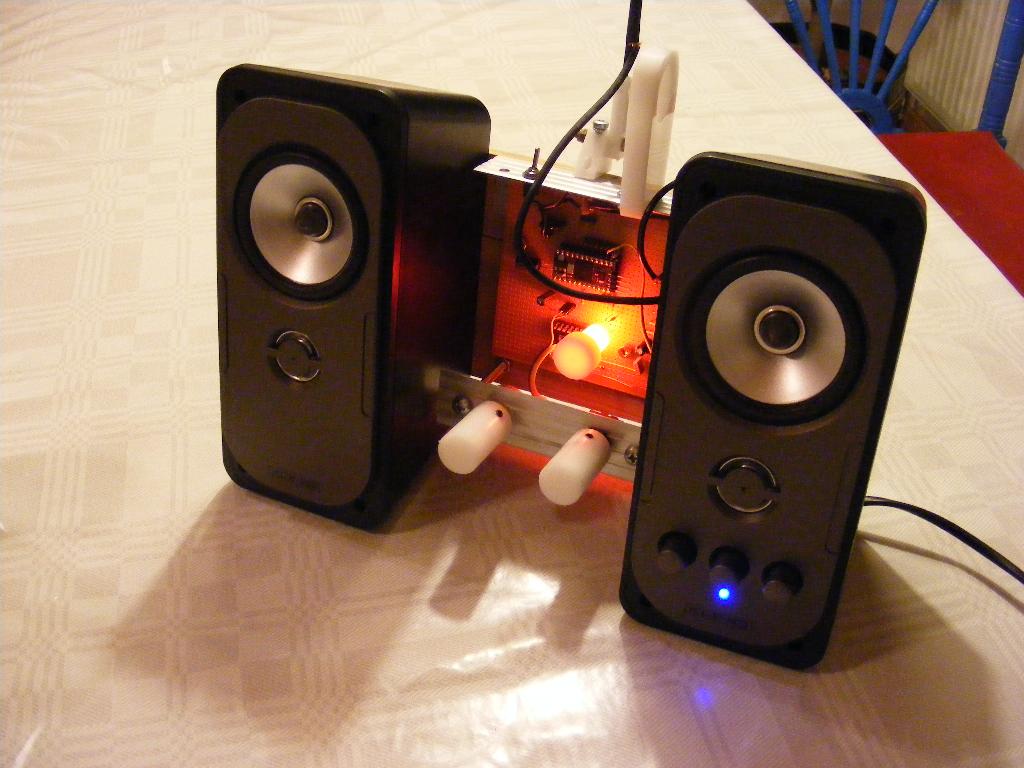
I bought a speaker system for a PC, and connected the
sound ouputs to them. I also broke my self into the
speaker, and borrowed 18 volts from the amplifier to
drive my computer and radio. Between the two speaker
boxes I put a piece of oak, on which I mounted the
electronics. The computer is a Spinstamp,
which is a surface mount Propeller computer together with
a crystal, EEPROM and voltage stabilizers in a hybrid
circuit. What remains is an A/D converter, a voltage
stabilizer for the radio, two pull up resistors for
the I2C bus and the radio itself.
Additionally I have connected an RGB led to the computer,
to show the choice of station. My family complained
about the strong light from the led, so I damped the
light with a plastic tube. The same material is used
for the knobs.
The antenna arrangement is not the easiest. The radio
chip has a single antenna input so I connected it to
a single rod. It's a normal copper wire attached to a
carbon fibre rod. The positioning of the antenna can
be critical where I live, so l made a joint for the
antenna rod with two degrees of freedom. A computer
with a working frequency of 80 MHz is a pretty good
disturbance source for an FM radio, but I tried to
shield the first decimeter of the antenna wire, and
to my surprise that worked.
Unfortunately, in the previous picture, you don't see
the radio itself. In this close up, you can see the
breakout board, though partly hidden by the shielded
antenna cable. Also unfortunately, the radio chip is
on the hidden side of the breakout board, so you don't
see it anyway. But you see the Spinstamp module.
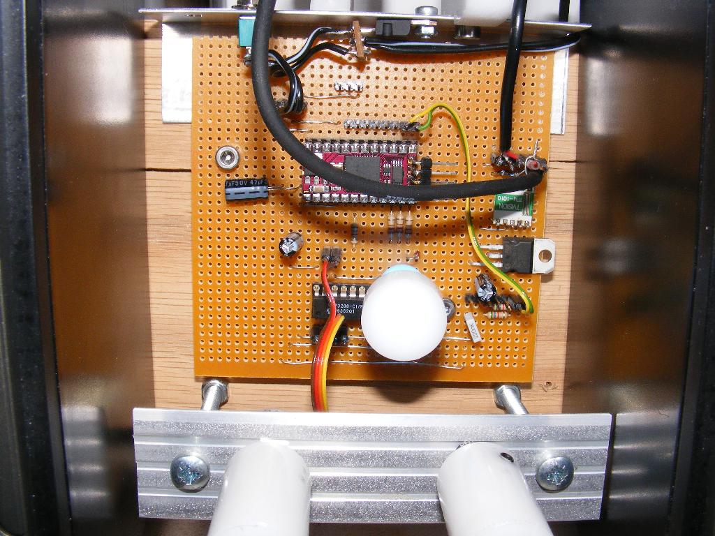
If I adjust the antenna position a little now and then,
I get excellent sound. Distortion is low, the audio
frequency range is excellent, my speaker amplifiers give
power enough, and I know I am always perfectly tuned.
Download radio.myo
Download radio.myr
Linear Camera
The linear camera is a little device from Hamamatsu
labeled S9227. It procuduces an image 512 x 1 pixel, so
it produces a one line picture. Another name is line sensor
or line scanner. I didn't know what I would use it for
when I bought it, and I still don't know. A use as a
robot sensor would be natural, but the vertical field of
view is quite small, so to use it for recognizing beacons,
you need either beacons of some height or a spread lens
in front of the sensor. In fact, the vertical pixel size
is 20 times bigger than the horizontal pixel size, but
the vertical pixel size is still quite small.
On the Parallax forum, there is someone who has taken
a sensor like this and mounted on a tilt table. Then he
can scan in a complete 2 dimensional image. He has even
put movable color filters in front of the camera, and thus
made a color picture. The exposure time is long, and the
colors are perhaps not perfect, but it's nice. You can
do it with this sensor and this software, if you just
make a tilt table. You have to accumulate the image in
a PC, because there is hardly enough memory onboard the
Propeller.
Nevertheless, I think this was a nice project. It's a
nice mixture of digital and analog technique, because
you clock in a video signal, that is analog in nature.
And with a single line, you can store the whole picture
in the Propeller, so you can build a stand alone solution
in a Propeller. With normal cameras you can hardly hope
to do that.
The sensor is just a sensor, so I made it a camera by
mounting it behind a magnifier. The focus of the magnifier
is such that I should mount the camera slightly behind
the backplane of the magnifier, so I used a sheet of
macrolone for that (plexiglass would do too). Then I
have an experiment circuit board and a connector and
cable, and that is all. Here it is, mounted on a
gorilla pod:
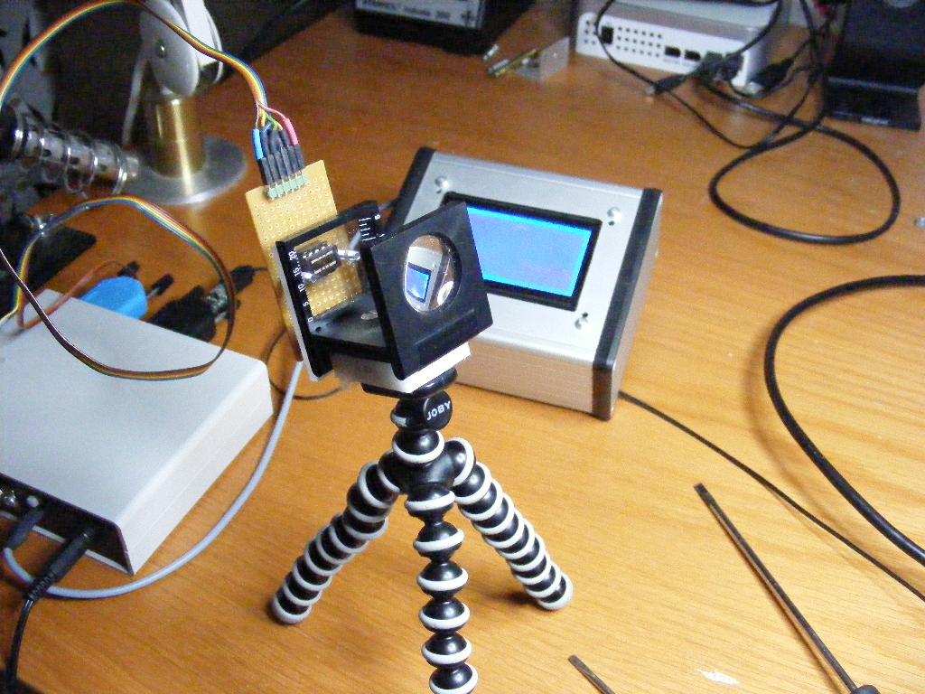
Here's a close up of the sensor:
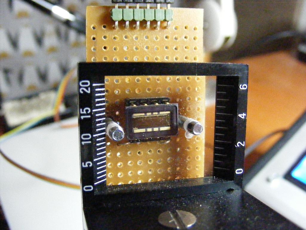
The software is a main program Lcam.myr, which captures
the image (process capt), displays it as a plot on the
graphical display (process show), and also sends image
data to a PC (process topc). The PC has to request the
data by sending an arbitrary byte, and then receives
512 bytes of image data.
For capturing, you could consult the spec. I don't include
it here, for I assume, that if you can get hold of the
sensor, you can get hold of the spec. You communicate with
the device with two pins, a startpin, and a clockpin.
When the startpin is high, you do the exposure. I preferred
to do that immediately after the previous picture was sent.
I use now an exposure time of 64μs. During transfer of a
picture, I keep the start pin low. You can transfer and
expose simultaneousy, but I chose not to use that.
For transferring, you should first send 15 clock pulses
to initialize the device. Then you run the clock signal up and
down, and then the next pixel is available, so you start
A/D conversion and fill your image array im. You
do this 512 times to get 512 pixels. Then you turn
the startpin on and continue to send clockpulses to expose
the next picture. (It is not clear to me, why you have to
send clockpulses to expose, but I tried without, and it
didn't work).
Here's the "picture" of a small lamp hanging in my window.
It is a little dark outside, so you only see the lamp.
The ambient light outdoors is undersaturated.
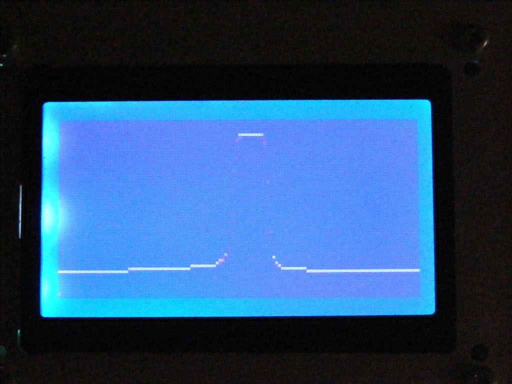
The Mandelbrot set
The Mandelbrot set is a set of complex numbers. Now,
as we have learnt here, a complex
number has two coordinates (the real and the imaginary), and
a point in the plane also has two coordinates, and thus
we can depict a set of complex numbers as a set of points
in the plane. So the set becomes a "figure" in the plane.
The Mandelbrot set was discovered by Bénoit Mandelbrot,
while he worked for IBM, but the Mandelbrot set has a
kind of dual relative, called the Julia set, discovered
by Gaston Julia and Pierre Fatou much earlier. But
Mandelbrot had the opportunity to make his set into
computer graphics, which quickly made it gain world
reputation.
The Mandelbrot set is generated from a very simple
equation (or rather function), but once it is there, and
you can show it with your computer graphics, and you can
zoom into its details, it reveals itself as an extremely
complicated structure.
Here is the function:
f(z) = z2 + c
z and c are complex numbers. What you do now, is
that you take what comes out of the function (f(z)) and
plug that back into z. And then you keep doing that. What
happens then? Well one of two things can happen, z can
stay limited, and maybe converge to something, or oscillate
in a limited world. Or, z can go to infinity. It depends
on what we start with, but we always start with z = (0,0)
= 0 + i·0 = 0. And it depends on the constant c.
Then, the Mandelbrot is the set of c-values, for which
z doesn't go to infinity.
To draw this, we start with some picture coordinates (ix,iy).
We map this with some linear mapping to a complex number
c = (cr,ci). Then we just run the
function iteration, and see what happens. We can't wait till
infinity for divergence, but the fact is that if divergence
happens, it happens pretty fast. Nevertheless, if we don't
wait long for divergence, then we miss some precision in our
drawing. OK, if there is no divergence, we draw a dot at
our picture coordinates, and then we go somewhere else.
The point now is, that by just changing the mapping from
(ix,iy) to c, we can effectively move around and zoom out
of and into the complex plane, and thus look for details
in the Mandelbrot set.
However, with fix point arithmetics, and 32 bits word length
(which is good enough for most purposes), it is hard to
give justice to the Mandelbrot set, so I recommend anybody
to repeat the experiment with, say, a Java program, where
the variables are represented as double precision floating
point values. In addition, you have a screen with higher
resolution.
But this Propeller program is a little feasability test,
which shows that you get a recognizeable Mandelbrot
set. Here's what it looks like with a real LCD screen.
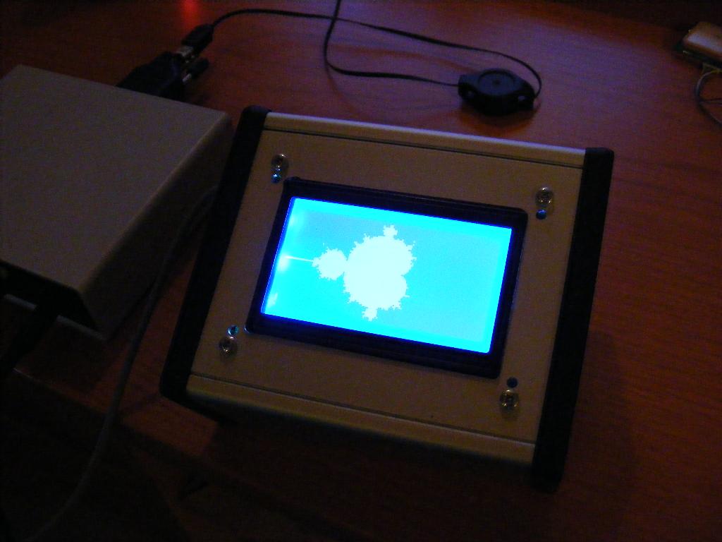
Download Mandelbrot.myr
Interfacing EEPROM
An EEPROM is an Electrically Erasable Programmable
Read Only Memory. A PROM is a memory with a content, that
you can give to it once and for all. An erasable Prom is
usually erased with UV lamp. After that, you can program it
again. An EEPROM is erased with an electrical signal, which
is handier than using a UV lamp. For the EEPROM:s I use
here, you don't really see a specific erase phase. They
behave as normal writeable memory (RAM or RWM), but they
keep the content after power down. However, the EEPROM:s
have a limited number of write cycles. After that, the
component is worn out. Depending on quality class, the
limit for the number of write cycles varies between
10 000 and 1 000 000. This is pretty much, but it makes
these components less suited for data logging, but well
suited for storing of programs.
Different types of memory cards, SD-cards, Memory sticks
etc. are popular components of this type, but it's hard
to find good documentation for them, and they have a
somewhat complicated structure (page structure). Ideally
you would like to implement a standard file system, so
that you can read and write data from a PC. I have a
device that does all this, based on a serial command
interface from a computer like a Propeller. But I didn't
always manage to erase files properly, it was somewhat
slow, and it is not sold anymore. (In Parallax' object
repository, there are Spin objects for handling SD-cards,
including building a file system for them).
EEPROM:s that look like ordinary electrical components
are also available. The upper limit in size is 1 MB,
but more will come, I suppose. The component type I have
chosen, is the type, that is used together with the
Propeller computer. The type is called 24LC256, which
has a size of 32 kB which is 256 kbits, hence the name.
With the same interface, a type called 24LC512 is
available. The size, consequently, is 64 kB. They can
be stacked together up to eight at a time, so then the
limit is 512 kB. If we store Propeller code, we are
interested in the number of long (32 bit) words, so then
the biggest chip contains 16 kLongwords. That's enough
to fill 32 Propeller cogs with code.
These devices are controlled through an I2C
interface. This is described here.
Since the eeprom application of I2C is somewhat
demanding, I have updated the assembler iic-routines,
so they are now in the state as described in
the I2C description.
24LCXXX memories have a memory page structure, but it
doesn't disturb too much. There is a page write
mode, but I haven't used it. My data to write are coming
from a PC over RS232, and if I were to write that data
one page at a time, I would have to store all that data
first in the Propeller RAM. It is possible, and faster
than writing individual bytes, but it is unnecessarily
complicated. You have the same situation if you want to
log real time data into the EEPROM.
For reading, you can read a single cell, but once you
have adressed that single cell, you can keep reading from
consecutive cells, and the limits between pages is
immaterial in this case.
For talking to the memory, your Propeller, as a master,
first has to wake up the device (the memory chip). It
does so by first sending a start pattern, and then a byte
with an I2C adress. The I2C adress
for these devices is always a hexadecimal A. After that
there are three bits, that allow you to adress up to
8 individual chips. The chips have three adress pins, and
you connect them to 1s and 0s in an individual pattern.
The chip that wakes up, is the one, whose wire pattern
matches the three bits sent. Finally, there is a receive/send
bit (0 for sending). To begin with, it is always 0,
because now you have to send a memory adress.This adress
takes up two bytes.
If you write data, you just keep sending the data after
the adress. When you are satisfied, you send a stop pattern.
In all this trafic, you have to leave the bus open between
the bytes, to allow the device to send an acknowledge bit.
When you want to read data, after the adress has been sent,
you send a start pattern and a new device adress, this time
with a 1 as receive/send bit. After an acknowledge bit,
you can clock in your data as long as you want, but you
have to acknowledge each byte received. Acknowledgment
amounts to sending a 0 on the bus.
I have a routine that reads a given number of bytes from
a specific EEPROM adress, to a given adress in an array
in Propeller RAM. I also have a routine that reads 4 bytes,
and then packs them into a longword. There is a consideration
there, about how the bytes in a word are supposed to be
packed into consecutive cells in a byte oriented memory.
The two principles here are called Big Endian and Little Endian.
It can be said that each of these principles is more logical
than the other (in some sense). Consequently Unix and
Windows have made different choices. I am not quite
sure what the alternative chosen in the Propeller should
be called, but I found the way the EEPROM content is
displayed in the Propeller Environment a little bit confusing.
Anyway, the code that you can download here works fine.
An External Program Memory
This is now my project for using the EEPROM.
When you use your Propeller computer "in the field", but
want to run different applications on it, you find, that
you have to bring a PC with you, to switch application.
It would be nice to have a small memory box, that could
contain a bundle of programs, that you could choose between,
load into
the Propeller and run.
Technically, we build a card with
one or more EEPROM chips, and connect its two control signals
(called clk and sda) to two Propeller pins. We also need
some means to control which program to run. As I have
analog input channel free, I have chosen to use a
potentiometer for choice of program. The current choice is
displayed as a color on my RGB-led. So you need a little
table to pair the applications with a color. I also need a button
to confirm a choice, and it is connected to a Propeller
I/O pin.
The rest is software. I'll come back to the software for
writing the EEPROM in a while.
For running the program, the key mechanism is a Propeller
instruction called coginit. It appears both as a
Spin instruction and an assembler instruction, but I use
the assembler instruction. It has one argument, which is
a reference to a variable, called cogreg by me, which
contains three different arguments packed into different bits.
The first of them is the number of the cog to be
started. The second is an adress to a cell in the
Propeller RAM, where the cog program is stored. The third
argument is an in principle arbitrary reference, that the
cog is provided with, so that it can find its way to global
variables.
Before we can use this, we have to load the program code
from the EEPROM into an appropriate place in Propeller RAM.
In fact, we load all the cog programs first into RAM before
we call coginit for all the cogs, in order to make all the
cogs start with reasonalbe simultaneity. We call the
whole program a Bootloader. The Propeller already has a
bootloader, but its implemented in ROM, so we can't modify
it for our purposes. Hence we have to let the built in
bootloader load our bootloader. It has to do so in a new
cog (number 1), so we waste one cog on this. From this,
our bootloader loads the remaining cogs from EEPROM via
RAM.
A cog has an adressable space of 512 longwords, but the
the sixteen last of these are special registers. Some
of these may be proper memory cells, but some are certainly
more general registers, which are mapped to the memory
adress space. The outa, dira and ina
registers are here. The first of them, which has some
importance here, is the paramater register par.
This register is loaded with content by the coginit
instruction, and the content is usually used as a way
to reach global variables in RAM. But the par register
is interesting for another reason. The bootloader loads
the program code into an array called ee. We should
give the adress of this array to coginit. But what we need,
is the absolute adress of ee. How do we find it?
Well, when we start our bootloader, from the standard
bootloader, we can write (in Spin now)
coginit(1,@boot,@ee). This should load the absolute
RAM adress of ee into the par register. So when
we call coginit to load our programs, we can compute
where the code is by adding the content of par and
some relative adress of the code within ee.
When we run our programs, once we have loaded them, we
would like to use the space taken up by ee for global
variables.
So the third part of the cogreg variable is also
based on par.
There are two more details in this to consider. Firstly,
in the bootloader, we need a few global variables except
ee, and it is easiest to put them first. Hence, the
par register doesn't contain exactly the adress
of ee, but it can be computed. Secondly, the
par register is 16 bits long, so that it can adress
every byte in RAM. But in cogreg, there is a lack of space,
so the 2 LSB's or the adress are shifted out. In this
way, we can still adress every longword in RAM. But we have
to do this shifting, when we load cogreg from
par.
Programs for the individual cogs are loaded both in the
EEPROM and RAM with a spacing of 512 longwords. These programs
are maximum 496 longwords, and minimally much smaller, so
there is some waste, but it is not too bad.
You will find the program Boot.myr
and the objectfile Eeprom.myo below.
Packing the bundle
The code you load into the program bundle in the EEPROM
is machine code, so I first had to make a machine code
generator. With the structure of Propeller Assembler, it
isn't awfully difficult. It produces the machine code
disguised as assembler code, so that all instructions are
presented as variable declarations, with data initalized
in binary form (following a %-sign). Hexadecimal code is
also presented as a comment on each line. Then there are
four initial lines, which makes the code runnable from
the Propeller environment.
The machine code generation is an integrated part of the
Myra system. In Myra.java there is boolean
machineCode that you can set to false if you want
normal assembler language code. In either case you can
procede through the Propeller Environment as usual, if
you want to run the program directly.
If you get mystified by the machine code, there is a
disassembler, that converts the code back to assembler.
The next step, if you want to make an eeprom bundle, is
to make a packlist, called packlist.txt. It has
a little code for writing a header in the eeprom. On
the packlist there is:
- A number, on the first line, which points
out the program to run
- Lines like Mandelbrot:3,2, where
"Mandelbrot" is the name of the application,
3 is the 512 longwords block where the
program starts. This figure is not zero.
2 is the number of cogs used.
This header part ends with a line with a number of
dashes ("----"). The rest of the packlist is just
a list of all the spin-files that go into the bundle.
They should be generated by Myra.java with the boolean
machineCode set to true. Currently the header
information is not used. I found it easier to write
this information into the bootloader Boot.myr.
Given this, you can run PackProm.java, which will generate
a machine code file, called eeprom.txt. This
represents all the machine code in a "readable"
hexadecimal format on a text file.
Next, one starts a program eeprog.myr in the
Propeller, and then one starts the Java program
PromWriteH.java. This will send over the file
to the Propeller, which will unpack the hexadecimal format,
and then store the bytes in consecutive cells in the
EEPROM.
Finally, you can look at the packlist file, and update
two arrays in Boot.myr. i0s contains the numbers
of the 512 blocks, where the application starts.
ncogs contains the number of cogs used by each
application.
Now you can load Boot.myr into the Propeller with the
Propeller Environment. If it works, you should also load it
into the Propellers standard EEPROM. Then, when you reset
the Propeller, some color will light up. You can turn
the knob to get the other colors. When the desired color
lights up, you press the button, and your program will
start.
Downloads
These are files to download. For the files from
PromWriteH.java and down, you can find more information
here.
Flash memories
Probably, the EEPROM memories we have just mentioned,
are flash memories. But they are really pretty small.
On the other end of the scale, we have the memory cards,
like SD cards and so on. They have a huge capacity, but
I find them difficult to program. In between there are
flash memories, which look like ordinary integrated circuits.
SST25VF032B is such a memory with a capacity of
4 MByte. It is delivered in a 8 pin SOIC surfacemount
package. The interface is serial, according to a standard
called SPI (Serial Peripheral Interface).
You can adress
individual bytes, and read or write them. But
you have to erase the byte before you can write it. But
you can't erase single bytes. You can only erase whole
blocks of memory (the blocks are called sectors by
the manufacturer). This needs to be considered, when
you write the memory. Erasing amounts to that all the
bits in the byte become 1 (so the bit pattern is
11111111 or FF in hexadecimal notation). Writing amounts
to lowering some bits to 0. So if you write more than
once to a byte, the result will effectively be a logical
and-ing of the words you try to write.
These memories have a very elaborated write protection,
system, so if you don't work hard, you have actually bought
yourself a read only memory, that you can't even program.
It is not easy to override this write protection, and you
wouldn't believe that you had been successfull, unless
you had actually tested it. Here are the protection
mechanisms:
- In order to lift the software write protection
mechanisms, you first have to lift a hardware
write protection in the form of a #WP-pin. Make it high
on the circuit board.
- Whenever you want to write something or
erase a block, you must first issue a
Write Enable-command.
- Then, there is a status register, and some
of its bits block parts of the memory. If
the bits are all 1, the whole memory is
write protected. And this is the value
the status register gets at power up.
- So you have to write to the status register
with a WRSR instruction. But this instruction
is blocked, unless it is immediately preceded
by a EWSR (Enable write status register) instruction.
Perhaps a Write Enable command is also
necessary before EWSR-WRSR.
The SPI protocol is built around 4 wires connecting
the memory and the computer:
- A clockline, which clocks commands and data
to and from the memory.
- A tristate output line, which sends data from
the memory (in the Myra code this is called
"di" as the thing is seen from the point of
view of the computer).
- A data input line.
- A chip enable line with negative logic.
Activities, which the memories should do
internally, are started from the moment that
the chip is disabled, i.e. the chip enable
line goes high.
Using these lines, one first sends a command to the
memory. Usually it is followed by three adress
bytes. After that, one can send data to, or receive
data from the memory using the four wires.
If the memory gets a task to do, one can monitor the
job using the status register, which can be read at
any time, or one can wait a fixed time. Writing a
byte takes 10μs. Erasing a block (sector) takes 3ms.
I chose to view this memory as a longword memory, i.e.
a memory where groups of four bytes make up a longword,
adressed with a longword adress, which moves one
longword, i.e. 4 bytes, when incremented with one.
The file flash.myo contains functions for this:
- fl.init for initialization. It is called
with pin numbers; dopin (data out to the memory)
dipin (data in), clkpin and cepin on the stack.
init sets up the pin numbers and initializes
the SPI communication.
- fl.inits, is an initialization with pin numbers
for a standard hardware configuration. inits
is called with the stack empty. It loads the
appropriate numbers on the stack and calls
init.
- fl.open opens the memory write protection
system. It has to be called after power up
(after init) to make the memory writeable.
- fl.erase is to be called with a longword
adress on the stack. It erases the memory sector
that contains that adress. The whole sector
will be erased to all 1's.
- fl.cherase with the stack empty, will
erase the entire chip.
- fl.write shall have a longword adress
on the stack, and under that a longword of data.
The data will be written to the adress.
- fl.read shall have a longword adress
on the stack, and will deliver the longword
from that adress of the memory
Furthermore there is a fl.bwrite and a fl.bread function
for writing and reading of a single byte. The byte
is placed in the least signifant byte of a longword,
and the adresses shall be byte adresses. There is
also a status register read instruction, fl.status,
to check if the write protection has been successfully
removed. In that case, the function should return 0.
The write enable function, which is used by other
functions is also available as fl.wren.
Download
A File System
On top of the flash.myo system, I've built an
object called file.myo, which represents a file
in a file system. You can create up to 5 instances of
the file object at the same time. They are distinguished
by a unit number, so any call to any of the
file functions should be preceded by the right unit number,
so that you work on the desired file. This allows you
to have 5 files open at a time, and move data between
them.
These files are the standard type files (not so called
random access files), where you stand at a pointer, and
can read or write data there, and then move the pointer
one step ahead.
Here's the main consideration for anyone who tries to
make a file system: You must imagine that you may
want to delete files.. If you have done that, there
is space left for new files. But if your new file is
bigger than the deleted one, you can't squeeze it in.
And if it is smaller, you get an even smaller piece of
space left. After a short time, the memory medium will
be like a Swiss cheese.
The remedy to this is fragmentation. You divide
your file into fragments of equal size. Now, when a
file i removed, you get a set of standard fragment holes
left over. Your new file's fragment fit precicely into
these holes. If the file is two big, there won't be enough
holes, so the new file will have to allocate its last
fragments elsewhere. It the new file is too small, some
holes will be left over for fragments of future files.
To make it possible to read through the file, each
fragments ends with a link to the next fragment of the
file. One says, that the whole file is represented
as a linked list.
In the PC world there is something called
defragmentation. It is not the opposite of
fragmentation, but a procedure to move the fragments
of each file as close as possible to one another,
physically. This is only meaningful for media like
magnetic discs, where one can avoid delays, when the
magnetic head has to move from fragment to fragment
over the disc.
The best choice for my memory, is to let a fragment
be as big as a memory block, i.e. 1024 longwords. It
is pretty much for a fragment, but it makes it easy
to erase files. As we delete a file fragment, we have
to erase the memory there, to make the area usable for
new files.
To find the start block of each file, we need a
file catalog to point out where each file begins.
Each entry in the filecatalog contains a file name,
and a starting block. I have chosen to represent
the block information with a single byte. Thus I can
only adress the first 255 blocks, but the remaining
blocks can contain fragments further down the files.
I have chosen to let the catalog entry for each file
be a single longword. That leaves only three bytes
for the file name. But it is good enough for my
purposes. I have also chosen to let my system contain
up to 64 files. That gives me a file catalog, which
is an array cat[] of 64 longwords.
I also need an account for which blocks are free in the
memory, and which are occupied. There are 1024 blocks.
which i 32x32 so we can store that information in
an array occ[] of 32 longwords.
cat[] and occ[] are placed in the first memory block.
However, they are not easy to work with there, as
you can't write to them without erasing the whole
block first. Hence, these two arrays have to be
mirrored into the Propeller RAM. At power up, you
read data to the mirrors from the flash memory. Then, basically,
you work with the mirror variables. But you should
see to that they get back to the flash memory every
now and then, so that no information is destroyed
at power down. You have a similar problem with a PC,
where you risk to loose information, if you just shut
power down. The system here writes the mirrored variables
back to the flash memory, after creation of any new file,
and after any delete operation.
Here's now a little of what you have to do:
- When you read a file, you have to observe
when you read the last cell in a block. At that
moment, you don't read data but a link to the
next block. You have to move to that new block
before you read.
- When you write a file, you have to observe
when you have reached the last cell in a block.
Then you should use occ[] to find a free block,
write a link to that block, and then move
there, to write the data item.
- When you delete a file, you should follow
the links through the file, and erase all the
blocks used by the file, and you should
remove the file entry in the catalog
(Note that you actually erase data, when you erase a
file. In many other systems, you just remove links,
so that the data remain intact, until the memory space
is needed for new files. Hence a skilled engineer can
often recover files, even if they have been deleted.)
Here now, are the functions from the object file.myo,
which are of interest externally:
- f.grandreset erases the whole file system
and configures an empty file catalog. Use with
care of course, but you need it, when you have
plugged in a new memory chip.
- inits is made to initialize the system
(preserving all old files) for a standard
configuration. It will call fl.inits and
fl.open, which will open up the write protections.
- f.new. Called as name i [f.new],
it will create a new file with the given name,
and unit number i, for writing. There is
no warning if you use an already used name,
but you do get a new file with the same name.
When you open a file with that name, you
can't be sure which of the files you get.
- f.write. Called as data i [f.write],
it will append the data last in the file with
unit number i.
- f.close. Called as i [f.close],
it will append an end of file symbol to the
file with unit number i.
- f.eof will return the end of file
symbol on the stack. You can use it to check
for the end of file situation, when you read
a file. The four bytes of the end of file symbol
are the ascii codes for the characters
null,"e","o" and "f".
- f.open. Called as name i [f.open]
it opens a file with the given name and
unit number i, as a file to read from.
There are no warnings if the file doesn't
exist (has never been created with [f.new]).
You will just get words with all 1's when
you try to read it.
- f.read.Called as i [f.read],
it will deliver the next longword on the
file to the stack.
- f.del. Is called with the name,
rather than the unit number, hence
name [f.del]. It will delete the
file with the given name, and leave the
used space free for new files.
Internally f.occupy, f.free
and f.freeblock mark blocks as occupied or
free and deliver the number of a free block.
And we have f.readcat and f.writecat
to move the file information between the flash
memory and the mirror in Propeller RAM.
Download
Interpretive Myra
The upside of an interpretive version of Myra is that
one avoids the limit of 496 longwords in Cog RAM. The
program resides in the global RAM of the propeller, where
there is much more space. From there, instructions are
loaded down to a cog and executed there.
The downside is that the execution is slower, firstly
because all the instructions have to be moved from the
global RAM to the cog, which takes a little longer time.
Secondly, the interpreter has to work a little with the
instructions, before they are executed. In practice, I
have observed a reduction in speed of 2 to 3 times, which
for many applications doesn't matter too much. (This is
the relation between compiled Myra, and interpreted Myra;
what you can do with hand written assembler code is
another matter).
Here's then how it works. You load each cog with an
interpreter, which is called Tolk.asm, from 'tolk', which
is Swedish for 'interpreter'. This interpreter, together
with the Propeller Cog, behaves in a new way relative to
the Propeller itself, so we can call it a virtual machine
Hence we can program this virtual machine in a new
language, which comes both as a somewhat readable
Assembler language, and as machine code. We call this
language iMyr.
The iMyr code is generated
from the Myra code, with a special compiler.
Hence, both compiled execution and interpretive execution
are compatible with the original Myra language. However,
interpretive execution has some advantages, and if we
use them, we may create a Myra program, that can't be
executed in compile mode. There are four major such
differences:
- As mentioned, the programs can be bigger in
interpretive mode
- In "immediate mode", when we push a value
directly on a Myra stack, we are limited by
the Propeller instruction format to numbers
below 512, while in iMyr, the limit is 224
(it is a limit in the iMyr instruction format).
- The iMyr virtual machine has a real subroutine
stack (of limited size though), which can allow
for a limited use of recursive calls.
- The
virtual machine also has a status stack, which
allows for a safer use of conditional statements.
The interpreter Tolk.asm is almost the same in every
cog in the application, but not quite. After we
have modified the interpreter, for each individual
cog, we call it a "Cog bundle". Making a cog bundle
(which is made by the iMyr compiler) amounts to the
following:
- The interpreter proper, is put in place. It
comes from a file called Tolk.asm, which is
written in Propeller Assembler. Comment lines
in this code are removed.
- On the second adress in the interpreter code,
there is a variable called base, which
points at the first iMyr instruction in the code
for this cog. So the initialization of base
is changed relatively to the code in Tolk.asm.
- The program can use local variables (the way
this is written in the Myra code). These
variables reside in the Cog RAM together with
the interpreter, so space has to be reserved
for them, and they need to be initialized, if
initial values are given in the Myra code.
- The user can call assembler routines in the
Myra code. These assembler routines differ
slightly from the assembler routines on the
Myra assembler resource file. They are found
in the file Assembler.asm and are loaded
from there into the space after the interpreter,
and the local variables. Hence, there is
a limit to how many and how big assembler routines
you can use in each process. After the
assembler routines have been put in place,
the compiler places a jump ladder in the
interpreter, so that the assembler routines
can be reached easily.
In interpretive mode, it is possible to initialize
global variables. This can be done in compiled mode
as well now, but with some limitation. These so called
data blocks can be used for things like font tables,
parameter lists etc.
The result of compilation is now a text file with
code given in a hexadecimal format (as lines of
8 hexadecimal figures). After the 8 hexadecimal figures,
there follows comment code which explains what the
8 hexadecimal figures represent, but which is ignored
by the computer. This file consists of the following.
- Data blocks
- Cog bundles for each of the cogs used
- iMyr machine code.
Each of these groups starts with an adress, where the
code is to be placed in global RAM, relative to the adress
of a huge array called ee[]. Each group ends with an
end code, which is hexadecimal 55555554, but the last
group ends whith a stop code, 55555555.
Instruction format
An iMyr instruction is parsed into three parts:
- The instruction type occupies 5 bits.
There are 24 types of instructions, so 5 bits
gives some spare.
- The condition occupies 3 bits.
There are 5 types of conditions, so, again,
there is som spare.
- Tre adress part takes up the rest of
the 32 bits. Adresses can be adresses to
local variables in the cog. The adress space
there i 9 bits (512 values). Adresses can
be adresses to the global RAM. We reserve
1024 longwords for global variables and data
blocks (which is the same thing here).
Adresses can also be target adresses for jumps.
They refer to adresses among the iMyr instuctions,
where 0 refers to the first instruction for the
cog in question. In immediate mode, the adress
part is just the value that is loaded to the
stack. We can load values up to 224,
which is a lot. For some instruction types,
the adress part further specifies what the
instruction does. Finally, for some instruction
type, the adress part doesn't mean anything
at all.
Some operations in the table below have names like
lmnop. These take m values from the stack, and
then present a result as n numbers on the stack. In
some cases, n=0, and in that case, the operation only
has side effects. For all these operations, the
adresspart decides what the operations do concretely.
| Code | Instruction | Description |
|---|
| 0 | pushim | push the adresspart to the stack top |
| 1 | push | push the value of the adressed
local variable |
| 2 | pushg | push the value of the adressed
global variable |
| 3 | pop | pop the stack top value to the
adressed local variable |
| 4 | popg | pop the stack top value to the
adressed global variable |
| 5 | pushel | For the following 4 instructions,
the stack top value is an index pointing to an array
element. The array base adress is the adress part
of the instruction. For this instruction, the
array resides in local memory. The value of the array
element is pushed to the top of the stack. |
| 6 | pushelg | Like the previous, but
the array resides in global memory. |
| 7 | popel | The next highest element
on the stack (i.e. under the index) is pushed
to the adressed array element in local memory. |
| 8 | popelg | Like the above, but
the array resides in global memory. |
| 9 | pushat | The two top elements on the
stack are summed, and the value at that adress in
local memory is pushed. |
| 10 | popat | The two top elements on the
stack are summed, and the third element on th stack
is popped to that adress |
| 11 | raise | raises the stack pointer,
so that a value popped off at a recent pop operation,
becomes visible again. |
| 12 | popoff | removes the top value
of the stack, whithout sending it anywhere |
| 13 | flip | exchanges the two top
elements on the stack with one another |
| 14 | dup | duplicates the top value
on the stack over the current stack top |
| 15 | jmp | A jump. The adress part is the
target of the jump |
| 16 | call | A subroutine jump. The
adress part is the target of the jump. This target
adress is pushed on the subroutine call stack. |
| 17 | return | This is a pop of the
subroutine stack. The value that is popped
up to the top of the stack is incremented with
one. |
| 18 | asm | calls an assembler routine.
The adress part selects which of the assembler
routines is called. |
| 19 | status | pushes the values of
the Propeller status registers (z and c-register)
on the status stack |
| 20 | rstatus | pops the status
stack, so that the previously sampled value
of the Propeller status is recovered. |
| 21 | l21op | Operation stack to stack |
| 22 | l11op | -"- |
| 23 | l01op | -"- |
| 24 | l10op | -"- |
| 25 | l20op | -"- |
Pushat and popat are used, when one wants a
subroutine that can operate on any array, rather than
a fix array. The array is pointed out through its adress.
These instructions are only available for local memory,
Here are the different lmnop-instruction as functions
of the adress part.
| l21op | - |
|---|
| 0 | + (addition) |
| 2 | - (sutraction) |
| 4 | or (logical or) |
| 6 | & (logical and) |
| 8 | xor (exclusive or) |
| 10 | >>n (non algebraic right shift) |
| 12 | >> (algebraic right shift) |
| 14 | << (left shift) |
| 16 | * (multiplication) |
| 25 | receive |
| l11op | - |
|---|
| 0 | || (abs) |
| 2 | compl (bitwise complement) |
| 5 | neg (negate) |
| 7 | G (1 if stack top greater than zero) |
| 11 | Z (1 if stack top is exactly zero) |
| 15 | inpin |
| l01op | - |
|---|
| 0 | inall |
| 2 | now |
| l10op | - |
|---|
| 0 | wait |
| 4 | setdir |
| l20op | - |
|---|
| 0 | outpins |
The virtual machine
Here's a simple sketch of the virtual machine.
In the middle of the figure, there is a register called
Instr Adress. Through the global RAM (gRAM),
the instruction is brought to the instruction register, where
it is parsed into type, condition and adress.
The type goes a little everywhere. The adress may go to the
memories (the global and the local) In case of a jump,
it goes to the Instr Adress register. This register is
connected to th subroutine call stack. In case of a
normal jump (jmp), nothing happens with this stack. In case
of a subroutine call, the previous value in the Instr Adress
register i pushed down into the call stack. When the stack is
popped, the value, that goes up to the Instr Adress register
is incremented with one. This means that execution
continues at the instruction after the subroutine call.
To the left is the normal stack, which communicates via
its top element with local or global memory. Some of the
memory cells in local memory (cog RAM) are mapped to
input and output registers, so this is how the computer
communicates with the outer world. Operations take data
from the highest layers of the stack, and push the results
to the top of the stack.
The status stack is depicted as a horizontal bar, as it
is actually a single memory cell, where status data
are shifted in. The least significan bits are updated from
the Propeller status registers, upon execution of a
"?" instruction (STATUS instruction). Subroutines that
use the "?" instruction, should restore the status
by popping the status stack with a "!" instruction.
Based on the condition and the value of the status stack
the condition checker decides whether the instruction shall
be executed or skipped.
Running interpretive Myra
As with Spin, there are two ways to run iMyr code;
directly from the PC or via the EEPROM.
For direct running,
we first have to bring a bootloader into the Propeller,
using the standard Propeller system. That bootloader is
called BootI, where "I" stands for this mode of running
iMyr. BootI will load the program into RAM, and then load
it further into the Cog memories with coginit as described
above. The file iMyrLoad.bat is a suggested
batch file, to make this as easy as normal execution of
Spin code. As easy - but a little slower, as the speed
is limited by the RS232-link with a speed of 115200 baud.
Also, the operator has to operate a "reset off" button,
to disconnect the reset of the Propeller chip from the
Prop stick device. Otherwise, the Propeller may reset, as
data come from the PC.
For running via EEPROM, we first need more EEPROM space,
than in the normal system. Replacing a 24LC256 chip with
a 24LC512 chip will do, and this causes no further work.
Alternately we can add an extra 24LC256, and connect
its adress pins to something other than (0,0,0). Then
we will load the loader EEPROG into the Propeller.
To control where the program goes into the EEPROM, we
should have an eeprom directive somewhere in
the source code file. It typically reads:eeprom:0,17.
0 is the EEPROM chip number. If we replace the 24LC256
chip with a 24LC512 chip, nr 0 is appropriate. If we have
more chips, and we want to use them, we direct the code
to them with some other number than 0. The figure 17
points out a 512 longwords big block in memory. For
24LC512, there are 32 such blocks. For chip 0, 16 blocks
are reserved for the ordinary Propeller system.
Compiling the Myra source code with the MyrI compiler
gives an .eep-file, which is loaded into the
EEPROM.
Running the code requires another program, BootJ,
where J stands for this EEPROM-mode. BootJ can be loaded
in the Propellers standard EEPROM, so that everything
starts at power up. BootJ has to be programmed so that
it loads the program from the correct block in EEPROM.
In the example above, a variable iblock should be
set to 17. You can use hardware jumpers, switches,
or potentiometers and A/D-converters, to allow different
applications to be ran at start up.
Downloads